Linear Programming Models for Traffic Engineering Under Combined - PowerPoint PPT Presentation
Linear Programming Models for Traffic Engineering Under Combined IS-IS and MPLS-TE Protocols D. Cherubini 1 A. Fanni 2 A. Frangioni 3 C. Murgia 4 a 3 P. Zuddas 5 A. Mereu 2 M.G. Scutell` 1 Tiscali International Network 2 DIEE - University of
Linear Programming Models for Traffic Engineering Under Combined IS-IS and MPLS-TE Protocols D. Cherubini 1 A. Fanni 2 A. Frangioni 3 C. Murgia 4 a 3 P. Zuddas 5 A. Mereu 2 M.G. Scutell` 1 Tiscali International Network 2 DIEE - University of Cagliari 3 DI - University of Pisa 4 Tiscali Italia 5 DIT - University of Cagliari October 8, 2008
Part I Introduction and Background
Problem Description Scenario Very large scale networks have been built by the Network Engineers Experience and Best Common Practice Planning Reaction to critical Network Events
Network survivability Techniques Network Design and Capacity Allocation Traffic Management and Restoration
Autonomous System (AS) Collection of IP Networks and routers controlled by a single administrative entity Two routing protocols End System-to-Intermediate System (ES-IS) Intermediate System-to-Intermediate System (IS-IS) IS-IS: link state routing protocol
Interior Gateway Protocol IS-IS/OSPF Metric associated to each arc Route selection using Dijkstra’s Shortest Path Algorithm Equal Cost Multiple Paths (ECMP)
MPLS Technology MPLS-TE Allows the configuration of the traffic in order to optimize the resources. Allows the building of VPN (Virtual Private Networks), using LSP (Label Switched Paths)-Tunnels . Extends existing IP protocol
Restoration Schemes: Link Restoration Figure: Link Restoration for single failure condition
Restoration Schemes: Path Restoration Figure: Path Restoration for single failure condition
Failure Analysis 20% : scheduled network maintenance activities 80% : unplanned failures where : 30% shared link failures 70% single link failures
Problem Statement Is it possible to obtain a robust configuration of the network using the combination of IS-IS routing and MPLS-TE techniques? Is it possible to formulate the question as a pure LP problem?
Linear Programmin Models min c · x A · x = b x ≥ 0 Graphs and Network Flows Generally, in Operations Research, the term network denotes a weighted graph G = ( N , A ) where the weights are numeric values associated to nodes and/or arcs of the graph.
Linear Programmin Models min c · x A · x = b x ≥ 0 Graphs and Network Flows Generally, in Operations Research, the term network denotes a weighted graph G = ( N , A ) where the weights are numeric values associated to nodes and/or arcs of the graph.
MMCF Problem Definition Notation G = ( N , A ) where N is the set of nodes and A ⊆ N × N is the set of arcs K is the set of commodities h − th commodity determined by: ( d h , s h , t h ), where s h ∈ N and t h ∈ N , with s h � = t h , are the starting and ending node, and d h is the quantity to be moved from s h to t h Formulations node-arc formulation : the variables are x h ij arc-path formulation: the variables are f p
MMCF: Node-arc formulation The problem ( i , j ) ∈A c h ij · x h min � � h ∈K ij − d h i = s h ( j , i ) ∈B S ( i ) x h ( i , j ) ∈F S ( i ) x h d h i = t h � ji − � ij = 0 otherwise h ∈ K x h � ij ≤ u ij ( i , j ) ∈ A x h ij ≥ 0 ( i , j ) ∈ A | N || K | + | A | constraints | K || A | variables
MMCF: Arc-path formulation The notation P h : the set of paths in G from the node s h to the node t h P = ∪ h ∈ K P h : the set of all relevant paths p ∈ P belongs to a unique commodity, identified by the starting and ending nodes of p ; h ( p ) c p = � ( i , j ) ∈ p c ij cost of the path p The problem min � � p ∈P h c p h ∈K = d h � h ∈ K p ∈ P h f p � p :( i , j ) ∈ p f p ≤ u ij ( i , j ) ∈ A ≥ 0 p ∈ P f p
Column generation.1 The problem has | A | + | K | constraints
Column generation.2 Let’s consider a reduced set of paths B ⊂ P . P B D B min c B f B max λ u + γ d ≤ u A B f B ≤ c B λ A B + γ E B E B f B = d ≤ 0 λ ≥ 0 f B
Column generation.2 Let’s consider a reduced set of paths B ⊂ P . P B D B min c B f B max λ u + γ d ≤ u A B f B ≤ c B λ A B + γ E B E B f B = d ≤ 0 λ ≥ 0 f B
Column generation.2 Let’s consider a reduced set of paths B ⊂ P . P B D B min c B f B max λ u + γ d ≤ u A B f B ≤ c B λ A B + γ E B E B f B = d ≤ 0 λ ≥ 0 f B
Column generation.3 If we solve the master problem we obtain: ˆ f B and (ˆ λ, ˆ γ ). Strong Duality: if (ˆ γ ) is feasible to DMMCF then ˆ λ, ˆ f B is optimal for MMCF Feasibility of the dual problem can be conveniently restated in terms of reduced cost of paths ˆ ( c ij − ˆ � � ¯ c p = c p − ˆ γ h ( p ) − λ ij = λ ij ) − ˆ γ h ( p ) . ( i , j ) ∈ P ( i , j ) ∈ P For all the paths p that belong to the set B we have that ¯ c p ≥ 0. What can we say about the paths p ∈ P \ B ?
Column generation.4 For each h ∈ K , we compute a minimum cost path from s h to t h by associating with each arc the new costs c ij − ˆ λ ij This minimum cost path is indicated by ˆ p h reduced cost of paths We compute the reduced cost ¯ c ˆ p h : if it’s greater or equal to zero for all h ∈ K : the set B holds the optimal paths If, instead, at least one path ˆ p h has negative reduced cost, then it can be added to B and the process is iterated.
Part II Models
LP MODEL with Node-Arc Formulation Data N - Node set A - Edge set F - Commodity set u ij - Capacity associated with link ( i , j ) d f - Effective bit rate of flow f x f ij - Share of flow f carried by IS-IS and traversing link ( i , j ) Variables u max - Maximum utilization in the network - objective function is f - Flow f carried by IS-IS flow f ij - Flow f carried by MPLS and traversing link ( i , j )
LP MODEL with Node-Arc Formulation Data N - Node set A - Edge set F - Commodity set u ij - Capacity associated with link ( i , j ) d f - Effective bit rate of flow f x f ij - Share of flow f carried by IS-IS and traversing link ( i , j ) Variables u max - Maximum utilization in the network - objective function is f - Flow f carried by IS-IS flow f ij - Flow f carried by MPLS and traversing link ( i , j )
Flows Aggregation Commodities aggregation by source node flow h � flow f ij = ij f : I ( f )= h Example Commodities A → B , A → C , and A → D are replaced by a single commodity “ A ”
Flows Aggregation Commodities aggregation by source node flow h � flow f ij = ij f : I ( f )= h Example Commodities A → B , A → C , and A → D are replaced by a single commodity “ A ”
General Routing Problem Objective function z = min( u max ) ij · is f + � f ∈F x f h ∈N flow h � ij ≤ u max · u ij ∀ ( i , j ) ∈ A f ∈ F ( h ) d f + is f − � i = h d f − is f j :( j , i ) ∈A flow h j :( i , j ) ∈A flow h � ji − � ij = if i � = h , i = E ( f ) , f ∈ F ( h ) 0 otherwise flow h ij ≥ 0 ∀ ( i , j ) ∈ A , ∀ h ∈ N is f ≥ 0 ∀ f ∈ F
General Routing Problem Capacity constraints z = min( u max ) ij · is f + � f ∈F x f h ∈N flow h � ij ≤ u max · u ij ∀ ( i , j ) ∈ A f ∈ F ( h ) d f + is f − � i = h d f − is f j :( j , i ) ∈A flow h j :( i , j ) ∈A flow h � ji − � ij = if i � = h , i = E ( f ) , f ∈ F ( h ) 0 otherwise flow h ij ≥ 0 ∀ ( i , j ) ∈ A , ∀ h ∈ N is f ≥ 0 ∀ f ∈ F
General Routing Problem Flow conservation equations z = min( u max ) ij · is f + � f ∈F x f h ∈N flow h � ij ≤ u max · u ij ∀ ( i , j ) ∈ A f ∈ F ( h ) d f + is f − � i = h d f − is f j :( j , i ) ∈A flow h j :( i , j ) ∈A flow h � ji − � ij = if i � = h , i = E ( f ) , f ∈ F ( h ) 0 otherwise flow h ij ≥ 0 ∀ ( i , j ) ∈ A , ∀ h ∈ N is f ≥ 0 ∀ f ∈ F
General Routing Problem Positivity constraint z = min( u max ) ij · is f + � f ∈F x f h ∈N flow h � ij ≤ u max · u ij ∀ ( i , j ) ∈ A f ∈ F ( h ) d f + is f − � i = h d f − is f j :( j , i ) ∈A flow h j :( i , j ) ∈A flow h � ji − � ij = if i � = h , i = E ( f ) , f ∈ F ( h ) 0 otherwise flow h ij ≥ 0 ∀ ( i , j ) ∈ A , ∀ h ∈ N is f ≥ 0 ∀ f ∈ F
General Routing Problem Positivity constraint z = min( u max ) ij · is f + � f ∈F x f h ∈N flow h � ij ≤ u max · u ij ∀ ( i , j ) ∈ A f ∈ F ( h ) d f + is f − � i = h d f − is f j :( j , i ) ∈A flow h j :( i , j ) ∈A flow h � ji − � ij = if i � = h , i = E ( f ) , f ∈ F ( h ) 0 otherwise flow h ij ≥ 0 ∀ ( i , j ) ∈ A , ∀ h ∈ N is f ≥ 0 ∀ f ∈ F
Link restoration
Survivability Constraints ij · is f + l − , l X x f , l X flow h X ( x l + , l · flow h · flow h ij + l + + x l − ) ≤ u max · c ij ∀ ( i , j ) � = l + , l − ∈ A ij ij f ∈F h ∈N h ∈N Share of flow carried by IS-IS when edge l fails Flow carried by explicit MPLS LSP along link ( i , j ) Share of flow flowing through edge l from node p to node q (arc l + ) and those from node q to node p (arc l − ) that is rerouted by IS-IS along link ( i , j ) Proof
Recommend
More recommend
Explore More Topics
Stay informed with curated content and fresh updates.
