Traffic signal optimization and traffic assignment Traffic signals - PowerPoint PPT Presentation
Dagstuhl, October 2015 Traffic Signals and User Equilibria Martin Strehler , Ekkehard K ohler BTU Cottbus-Senftenberg { martin.strehler,ekkehard.koehler } @b-tu.de Traffic signal optimization and traffic assignment Traffic signals Traffic
Dagstuhl, October 2015 Traffic Signals and User Equilibria Martin Strehler , Ekkehard K¨ ohler BTU Cottbus-Senftenberg { martin.strehler,ekkehard.koehler } @b-tu.de
Traffic signal optimization and traffic assignment Traffic signals
Traffic signal optimization and traffic assignment Traffic signals Traffic assignment traffic signals affect travel times road users may change routes combined traffic signal optimization traffic assignment problem
Traffic signal optimization and traffic assignment Traffic signals Traffic assignment traffic signals affect travel times road users may change routes combined traffic signal optimization traffic assignment problem traffic signals change over time need for dynamic traffic assignment
Challenges • traffic signal optimization is NP-hard • pseudo-polynomial time algorithms for multi-commodity flows over time (weakly NP-hard) • no constant-factor approximation algorithm for combined problem
Challenges • traffic signal optimization is NP-hard • pseudo-polynomial time algorithms for multi-commodity flows over time (weakly NP-hard) • no constant-factor approximation algorithm for combined problem on-going project (DFG grant) Optimization and network wide analysis of traffic signal control together with Kai Nagel, TU Berlin Primary objectives: Recent objectives • develop a linear model • system optimum vs. user equilibrium • focus on system optima • robustness, e.g., major events • solve it with mixed integer • public transport programming for medium-sized • . . . scenarios • validate solutions with traffic simulation
The cyclically time-expanded model Simple network t = 3 t = 3 t = 1 y x t = 2
The cyclically time-expanded model Time expansion (infinite time horizon) . . . . . . t 5 5 . . . . . . 4 4 3 5 3 5 2 4 2 4 3 3 1 1 2 2 1 1 y x
The cyclically time-expanded model Time expansion (infinite time horizon) . . . . . . t 5 5 . . . . . . 4 4 3 5 5 3 5 2 4 4 2 4 3 3 1 1 2 2 1 1 y x
The cyclically time-expanded model Periodic traffic signals → finite and cyclic expansion modulo T t 5 5 4 4 3 5 5 5 3 5 2 4 4 4 2 4 1 3 3 1 3 2 2 1 1 y x
The cyclically time-expanded model connect consecutive copies → waiting possible t 5 5 4 4 3 5 5 5 3 5 2 4 4 4 2 4 1 3 3 1 3 2 2 1 1 y x
The cyclically time-expanded model connect consecutive copies → waiting possible t 5 5 4 4 3 5 5 5 3 5 2 4 4 4 2 4 1 3 3 1 3 2 2 1 1 y x semi-dynamic or hybrid model
Modeling a traffic signal 7 6 5 4 3 2 1 0 t = 3 t = 1
Modeling a traffic signal 7 c 6 = b 6 c 6 c 5 = b 5 c 5 c 4 = b 4 c 4 c 3 = b 3 c 3 c 2 = b 2 c 2 c 1 = b 1 c 1 c 0 = b 0 c 0 t = 3 t = 1
Modeling a traffic signal 7 6 5 4 3 2 1 0 t = 3 t = 1
Modeling signalized intersections
Modeling signalized intersections
Modeling signalized intersections • collision free b 1 , i + b 2 , i ≤ 1 ∀ i ∈ { 0 ,..., T − 1 }
Modeling signalized intersections • collision free b 1 , i + b 2 , i ≤ 1 ∀ i ∈ { 0 ,..., T − 1 } • green length limitations t min ≤ ∑ T − 1 i = 0 b 1 , i ≤ t max
Modeling signalized intersections • collision free b 1 , i + b 2 , i ≤ 1 ∀ i ∈ { 0 ,..., T − 1 } • green length limitations t min ≤ ∑ T − 1 i = 0 b 1 , i ≤ t max • switching only once per cycle – new variables b on 1 , i – ∑ T − 1 i = 0 b on 1 , i = 1 – b 1 , i − b 1 , i − 1 ≤ b on ∀ i ∈ { 0 ,..., T − 1 } 1 , i
5 6 7 3 4 2 1 Figure: The Brunswick network with 5 signalized intersections (1–5) and two pedestrian signals (6,7). The three commodities under consideration are visualized with arcs in different colors. The underlying map was created with www.openstreetmap.org .
84 0 5B 4B 84 0 5A 3B 6 7 4A 84 0 1 2 3A 6 7 4A Figure: Optimized green bands for the Brunswick scenario. Time and state of the signals is shown on the vertical axis. Signals are labelled with intersection numbers and signal groups, e.g., signal 3 A and 3 B must not be green at the same time. Distances on the horizontal axis are chosen with respect to transit time, the slope of the parallelograms is chosen with respect to free speed. Note that the purple commodity is travelling from right to left and the cyclic overflow is visualized by a negative slope.
0 1 2 3 4 5 6 0 0 − 100 River Spree 7 100 − 200 19 20 21 200 − 300 8 300 − 400 400 − 500 18 22 23 9 500 − 600 24 17 600 − 800 29 > 800 25 16 26 28 30 27 15 31 14 10 11 13 12 Figure: Traffic assignment for the Cottbus scenario calculated with the cyclically time-expanded model (cars per hour and lane). The traffic on the outer road is increased in clockwise direction.
0 1 2 3 4 5 6 River Spree 7 19 20 21 8 18 22 23 9 24 17 29 25 16 26 28 27 30 15 31 14 10 11 13 12 Figure: Splitting of two commodities in the Cottbus scenario.
0 1 2 3 4 5 6 ≤ 5 5 − 50 River Spree 7 50 − 100 19 20 21 100 − 150 8 150 − 200 200 − 250 18 22 23 9 250 − 300 24 17 300 − 400 29 > 400 25 16 26 28 30 27 15 31 14 10 11 13 12 Figure: This diagram shows the waiting time integrated over all cars during one cycle at each traffic signal after optimization with our model.
Flow-independent travel times? The cyclically time expanded model includes • constant transit time on each arc • cost = flow · transit time • objective: minimize total travel time
Flow-independent travel times? The cyclically time expanded model includes • constant transit time on each arc • cost = flow · transit time • objective: minimize total travel time Is this too simplifying?
Flow-independent travel times?
Flow-independent travel times?
Flow-independent travel times?
Flow-independent travel times? 17 16 average travel time 15 14 13 12 11 10 max capacity flow
Platoons Traffic signals cause varying traffic density, i.e., platoons of cars: • arrival time at intersections is important ⇒ coordination • traffic signals may create, split, merge, densify, or loosen platoons • actual travel time depends an various parameters, e.g., position within the platoon • average travel time also depends an several parameters
Platoons Traffic signals cause varying traffic density, i.e., platoons of cars: • arrival time at intersections is important ⇒ coordination • traffic signals may create, split, merge, densify, or loosen platoons • actual travel time depends an various parameters, e.g., position within the platoon • average travel time also depends an several parameters Link performance functions etc. are not suitable for capturing platoons.
Platoons in the cyclically expanded network
Computed travel time of a platoon 40 35 Average travel time 30 25 20 15 10 60 30 50 40 40 50 30 0 20 10 10 20 Arrival time 30 0 Platoon length average travel time of a car in a platoon with respect to platoon length (in flow units) and arrival time at the traffic signal (in seconds after beginning of green phase)
Simulation with VISSIM scenario in VISSIM • 30 s green, 30 s red • platoons of different lengths (i.e., different traffic flow) and low density arrive • narrow road becomes wider (more lanes) • first car may wait longest if it arrives at beginning of red • platoon is densified by signal
Simulation with VISSIM 30 25 Average Travel Time 20 15 10 5 0 0 10 20 30 40 50 60 Platoon Length computed travel time (first car arrives 10 seconds before green)
Simulation with VISSIM 30 30 25 25 Average Travel Time 20 Average Travel Time 20 15 15 10 10 5 5 0 0 0 10 20 30 40 50 60 0 10 20 30 40 50 60 Platoon Length Platoon Length computed travel time simulated travel time (first car arrives 10 seconds before green) (100 runs, 5 hrs simulated time each)
User equilibria in the cyclically time-expanded model in theory: • system optimum is user equilibrium (constant travel-times, no road user can switch to faster route → Wardrop condition fulfilled) • capacitated network → value of user equilibria not unique • price of anarchy unbounded in practice: • simulate user equilibria with MATSim • there is a difference between our solutions and MATSim equilibria • difficult to compare (structure of) solutions
What is a realistic equilibrium? ‘projected’ travel times ue with capacities • more cars may imply lower travel times – traffic signals setter – adaptive signals – ...
What is a realistic equilibrium? ‘projected’ travel times ue with capacities • more cars may imply lower travel times – traffic signals setter – adaptive signals – ... • nearly no theory for non-convex, non-monotone settings • easy to construct bad instances for the general case • what can be done with additional assumptions? • (but not suitable for optimization purposes in our model)
Recommend
More recommend
Explore More Topics
Stay informed with curated content and fresh updates.
