Sampling a Signal an analog signal together with some samples of - PowerPoint PPT Presentation
Sampling a Signal an analog signal together with some samples of the signal. The samples shown are equally spaced and simply pick off the value of the underlying analog value of the underlying analog signal at the appropriate times. If
Sampling a Signal an analog signal together with some samples of the signal. The samples shown are equally spaced and simply pick off the value of the underlying analog value of the underlying analog signal at the appropriate times. If we let T denote the time interval between samples, then the times at which we obtain samples are given by nT where n = . . . ,− 2 ,− 1 , 0 , 1 , 2 , . .
Sampling It is often convenient to talk about the sampling frequency f s . If one sample is taken every T seconds, then the sampling frequency is f s = 1 /T Hz. The sampling frequency could also be stated in terms The sampling frequency could also be stated in terms of radians, denoted by ω s . Clearly, ω s = 2 πf s = 2 π/T .
The sampler The type of sampling mentioned above is sometimes referred to as “ideal” sampling. In practice, there are usually two non-ideal effects. One effect is that the sensor (or digitizer) obtaining the samples One effect is that the sensor (or digitizer) obtaining the samples can’t pick off a value at a single time. Instead, some averaging or integration over a small interval occurs, so that the sample actually represents the average value of the analog signal in some interval. This is often modeled as a convolution – namely, we get samples of y ( t ) = x ( t ) h ( t ), so that the sampled signal is y [ n ] = y ( nT ). In this case, h ( t ) represents the impulse response of the sensor or digitizer. Actually, sometimes this averaging can be desirable. For example, if the original signal x ( t ) is changing particularly rapidly compared to the sampling frequency.
The sampler The second non-ideal effect is noise. Whether averaged or not, the actual sample value obtained will rarely be the exact value of the underlying analog signal at some time. underlying analog signal at some time. Noise in the samples is often modeled as adding (usually small) random values to the samples.
Signal Reconstruction Possible continuous-time functions corresponding to samples. Unless we have some additional knowledge or make some assumptions, this problem clearly has many solutions.
Possible reconstructions Nearest-neighbor Zero-order hold
Possible reconstructions first-order-hold (linear interpolation)
The reconstruction approach
The Sampling Theorem Sampling a sinusoid at a high rate:
The Sampling Theorem Sampling a sinusoid at too slow of a rate:
The Sampling Theorem if the original signal has frequency f , then we will be able to exactly reconstruct the sinusoid if the sampling frequency satisfies f > 2 f , f S > 2 f , that is, if we sample at a rate faster than twice the frequency of the sinusoid. If we sample slower than this rate then we will get aliasing, where the alias frequency is given by fa = |fs − f|.
How to avoid aliasing Even in the case where it seems we have no problem recovering the sinusoid, we can’t be sure that the true sinusoid is not one of a much higher frequency and we are not sampling fast enough. are not sampling fast enough. The way around this problem is to assume from the outset that the sinusoids under consideration will have a frequency no more than some maximum frequency f B . Then, as long as we sample faster than 2 f B , we will be able to recover the original sinusoid exactly.
Sampling in the frequency domain A signal x ( t ) is said to be bandlimited if there is some frequency ω B < ∞ such that X ( ω ) = 0 for |ω| > ω B To recover a sinusoid at frequency ω we need to sample at a rate at least 2 ω . Thus, as long as the various sinusoids can be treated independently, we might guess that for a bandlimited signal we would be able to reconstruct x ( t ) exactly if we sample at a rate above 2 ω B .
Sampling theorem A bandlimited signal with maximum frequency ω B can be perfectly reconstructed from samples if the sampling frequency satisfies ω S > 2 ωB or equivalently, if f > 2 f or equivalently, if f S > 2 f B
Signal reconstruction Multiplying the spectrum of the sampled signal by 1/ T rect[ ω/ (2 ω B )] in frequency domain we get X ( ω ). Then x ( t ) can be recovered by an inverse Fourier transform. It’s also useful to consider what operations are done in It’s also useful to consider what operations are done in the time domain in the process of recovering x ( t ). Recall that multiplication of two signals in the frequency domain corresponds to a convolution in the time domain – specifically, in this case a convolution of the sampled signal with the sinc function (since the Fourier transform of a sinc function is the rect function).
Aliased signal As with pure sinusoids, if a signal is sampled too slowly, then aliasing will occur. High frequency components of the signal will appear as components at some lower frequency. This can also as components at some lower frequency. This can also be illustrated nicely in frequency domain. If sampled too slowly, the replicas of X ( ω ) overlap and the Fourier transform of the sampled signal is the sum of these overlapping copies of X ( ω ).
Quantization Quantization makes the range of a signal discrete, so that the quantized signal takes on only a discrete, usually finite, set of values. Unlike sampling (where we saw that under suitable Unlike sampling (where we saw that under suitable conditions exact reconstruction is possible), quantization is generally irreversible and results in loss of information. It therefore introduces distortion into the quantized signal that cannot be eliminated.
Quantization With L levels, we need N = log 2 L bits to represent the different levels, conversely, with N bits we can represent L = 2 N levels.
Uniform quantization
Uniform quantization
Non uniform quantization
Uniform vs. non-uniform quantization
Recommend
More recommend
Explore More Topics
Stay informed with curated content and fresh updates.
