Likelihood-based estimation, model selection, and forecasting of - PowerPoint PPT Presentation

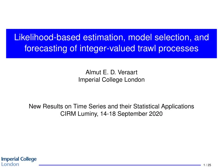
Likelihood-based estimation, model selection, and forecasting of integer-valued trawl processes Almut E. D. Veraart Imperial College London New Results on Time Series and their Statistical Applications CIRM Luminy, 14-18 September 2020 1 / 25

Collaborators This is joint work with ➤ Mikkel Bennedsen (Aarhus University) ➤ Asger Lunde (Aarhus University) ➤ Neil Shephard (Harvard University) 2 / 25

Introduction ➤ Time series of counts appear in various applications: Medical science, epidemiology, meteorology, network modelling, actuarial science, econometrics and finance. ➤ Count data: Non-negative and integer-valued, and often over-dispersed (i.e. variance > mean). ➤ Recently the class of (integer-valued) trawl (IVT) processes has been introduced as a flexible model, see Barndorff-Nielsen et al. (2014) for the univariate and Veraart (2019) for the multivariate case. Aim of the project ➠ Improve the estimation method for IVT processes (likelihood-based rather than moment-based); ➠ Tailor model selection tools to the IVT class; ➠ (Probabilistic) forecasting of IVT processes; 3 / 25

A very short and incomplete review of the literature ➤ Recent surveys & some new developments: Cameron & Trivedi (1998), Kedem & Fokianos (2002),Cui & Lund (2009); Davis et al. (1999); Davis & Wu (2009); Jung & Tremayne (2011); McKenzie (2003); Weiß (2008), Karlis (2016), Fokianos (2016). ➤ Literature on count data is spread across different disciplines. ➤ Overall, two predominant modelling approaches: ➠ Discrete autoregressive moving-average (DARMA) models introduced by Jacobs & Lewis (1978a,b). ➠ Models obtained from thinning operations going back to the influential work of Steutel & van Harn (1979), e.g. INAR(MA), see e.g. Pedeli et al. (2015). ➤ Further models: Regression type models (typically based on generalised linear models, see e.g. Fokianos (2016)), also Fokianos et al. (2020); state-space and Bayesian approaches. Our approach: ➤ Use ”trawling” for modelling counts. ➤ This is a continuous-time framework based on the idea of ”thinning” points. 4 / 25

Introduction What is trawling...? A first ”definition” “Trawling is a method of fishing that involves pulling a fishing net through the water behind one or more boats. The net that is used for trawling is called a trawl.” (Wikipedia) 5 / 25

Theoretical framework Definition of trawl process We define a stationary integer-valued trawl (IVT) process ( X t ) t ≥ 0 by � X t = L ( A t ) = R × R I A ( x , s − t ) L ( dx , ds ) . ➤ L is the integer-valued, homogeneous L´ evy basis on [ 0 , 1 ] × R : ➠ L ( dx , ds ) : = � ∞ − ∞ yN ( dy , dx , ds ) , ( x , s ) ∈ [ 0 , 1 ] × R . ➠ N is a homogeneous Poisson random measure on Z × [ 0 , 1 ] × R with compensator η ⊗ Leb ⊗ Leb , i.e. E ( N ( dy , dx , ds )) = η ( dy ) dxds , where η is evy measure satisfying � ∞ a L´ − ∞ min ( 1 , | y | ) η ( dy ) < ∞ . ➤ A Borel set A t = A + ( 0 , t ) with A = A 0 ⊆ [ 0 , 1 ] × ( − ∞ , 0 ] and Leb ( A ) < ∞ is called the trawl. ➠ Typically, we choose A to be of the form A = { ( x , s ) : s ≤ 0 , 0 ≤ x ≤ d ( s ) } , where d : ( − ∞ , 0 ] �→ [ 0 , 1 ] is continuous and Leb ( A ) < ∞ . 6 / 25

Example Poisson-Exponential trawl 1 0.8 0.6 0.4 0.2 0 10 11 12 13 14 15 16 17 18 19 15 15 10 10 5 5 0 0 10 10 11 11 12 12 13 13 14 14 15 15 16 16 17 17 18 18 19 19 7 / 25

Example Negative binomial-Exponential trawl 1 0.8 0.6 0.4 0.2 0 10 11 12 13 14 15 16 17 18 19 25 25 20 20 15 15 10 10 5 5 0 0 10 10 11 11 12 12 13 13 14 14 15 15 16 16 17 17 18 18 19 19 8 / 25

Some key properties of IVT processes Cumulants ➤ The IVT process is stationary and infinitely divisible. ➤ The IVT process is mixing ⇒ weakly mixing ⇒ ergodic. ➤ The cumulant (log-characteristic) function of a trawl process is, for θ ∈ R , given by C X t ( θ ) = C L ( A t ) ( θ ) = Leb ( A ) C L ′ ( θ ) , where the random variable L ′ (called the L´ evy seed) associated with L satisfies � � e i θ y − 1 � E [ exp ( i θ L ′ )] = exp ( C L ′ ( θ )) , C L ′ ( θ ) = η ( dy ) . with ➠ I.e. to any infinitely divisible integer-valued law π , say, there exists a stationary integer-valued trawl process having π as its one-dimensional marginal law. ➤ The autocorrelation function is given by . = Cor ( Y t , Y t + h ) = Leb ( A ∩ A h ) ρ ( h ) . for h > 0 . , Leb ( A ) 9 / 25

Examples Modelling the marginal distribution Example 1 (Poissonian L´ evy seed) Let L ′ ∼ Poisson ( ν ) . Then X t ∼ Poisson ( ν Leb ( A )) , i.e., for all t ≥ 0, P ( X t = k ) = ( ν Leb ( A )) k e − ν Leb ( A ) / k ! , k = 0 , 1 , 2 , . . . . Example 2 (Negative Binomial L´ evy seed) Let L ′ ∼ NB ( m , p ) for m > 0 , p ∈ [ 0 , 1 ] . Then X t ∼ NB ( m Leb ( A ) , p ) , i.e., for all t ≥ 0, P ( X t = k ) = Γ ( Leb ( A ) m + k ) k ! Γ ( Leb ( A ) m ) ( 1 − p ) Leb ( A ) m p k , k = 0 , 1 , 2 , . . . , where Γ ( z ) = � ∞ 0 x z − 1 e − x dx for z > 0 is the Γ -function. 10 / 25

Examples Modelling the trawl function/correlation structure ➤ Recall the typical choice for the trawl: A = A 0 = { ( x , s ) : s ≤ 0 , 0 ≤ x ≤ d ( s ) } , A t = A + ( 0 , t ) . ➤ Restrict attention to a class of superposition trawls : � ∞ e λ s π ( d λ ) , d ( s ) : = s ≤ 0 , 0 where π is a probability measure on R + . ➤ For h ≥ 0, the acf is given by � ∞ h d ( − s ) ds ρ ( h ) : = Cor ( L ( A t + h ) , L ( A t )) = Leb ( A h ∩ A ) = � ∞ 0 d ( − s ) ds . Leb ( A ) 11 / 25

Examples Modelling the trawl function/correlation structure ➤ Exponential trawl function: Let λ > 0 and π ( dx ) = δ λ ( dx ) , then d ( s ) = e λ s for s ≤ 0 and ρ ( h ) = Cor ( X t + h , X t ) = exp ( − λ h ) , h ≥ 0 . ➤ Inverse Gaussian trawl function: Letting π be given by the inverse Gaussian distribution π ( dx ) = ( γ / δ ) 1 / 2 � − 1 � 2 ( δ 2 x − 1 + γ 2 x ) 2 K 1 / 2 ( δγ ) x − 1 / 2 exp dx , where K ν ( · ) is the modified Bessel function of the third kind and γ , δ ≥ 0 with both not zero simultaneously. Then � � − 1 / 2 � � �� � 1 − 2 s 1 − 2 s d ( s ) = 1 − s ≤ 0 , exp δγ , γ 2 γ 2 � � � ρ ( h ) = Cor ( X t + h , X t ) = exp δγ ( 1 − 1 + 2 h / γ 2 ) h ≥ 0 . , 12 / 25

Examples Modelling the trawl function/correlation structure ➤ Gamma trawl function: Let π have the Γ ( 1 + H , α ) density, 1 Γ ( 1 + H ) α 1 + H λ H e − λα dx , π ( dx ) = where α > 0 and H > 0 . � − ( H + 1 ) 1 − s � d ( s ) = s ≤ 0 , , α and � − H ρ ( h ) = Cor ( X t + h , X t ) = Leb ( A h ∩ A ) � 1 + h = . Leb ( A ) α Note that in this case � ∞ � ∞ if H ∈ ( 0 , 1 ] , ρ ( h ) dh = α if H > 1 , 0 H − 1 i.e. the trawl process has long memory for H ∈ ( 0 , 1 ] . 13 / 25

Estimation From method of moments to composite likelihood ➤ Suppose we have n ∈ N observations of the IVT process X , x 1 , . . . , x n , on an equidistant grid of size ∆ = T / n . ➤ Define n − h CL ( h ) ( θ ; x ) : = ∏ f ( x i + h , x i ; θ ) , h ≥ 1 . i = 1 ➤ Let Θ be a compact parameter space such that the true parameter vector, θ 0 , lies in the interior of Θ . ➤ Construct the composite likelihood function, for H ⊆ { 1 , 2 , . . . , n − 1 } , n − h L H CL ( θ ; x ) : = ∏ CL ( h ) ( θ ; x ) = ∏ ∏ f ( x i + h , x i ; θ ) . h ∈H h ∈H i = 1 ➤ The maximum composite likelihood (MCL) estimator of θ is defined as θ CL : = arg max ˆ θ ∈ Θ l H CL ( θ ; x ) , where l H CL ( θ ; x ) : = log L H CL ( θ ; x ) is the log composite likelihood function. 14 / 25

Pairwise likelihood The general case and a simulation-based approach ➤ The joint probability mass function of two observations x i + h and x i is � � f ( x i + h , x i ; θ ) : = P θ X ( i + h ) ∆ = x i + h , X i ∆ = x i ∞ � � ∑ = P θ L ( A ( i + h ) ∆ \ A i ∆ ) = x i + h − c c = − ∞ � � · P θ L ( A i ∆ \ A ( i + h ) ∆ ) = x i − c � � · P θ L ( A ( i + h ) ∆ ∩ A i ∆ ) = c . evy basis L is positive, i.e. η ( y ) = 0 for y < 0. Then we ➤ Suppose the L´ min { x i + h , x i } can replace ∑ ∞ c = − ∞ by ∑ in the above formula. c = 0 ➤ Let t , s ≥ 0, choose C ∈ N and let c ( j ) ∼ L ( A t ∩ A s ) , j = 1 , 2 , . . . , C , be an iid sample. A simulation based unbiased estimator of f ( x t , x s ; θ ) is C f ( x t , x s ; θ ) = 1 ˆ P θ ( L ( A t \ A s ) = x t − c ( j ) ) P θ ( L ( A s \ A t ) = x s − c ( j ) ) . ∑ C j = 1 15 / 25

MCL outperforms GMM for IVTs 2 2 m p 1.5 1.5 1 1 0.5 0.5 0 0 0 2000 4000 6000 8000 0 2000 4000 6000 8000 2 2 m p 1.5 1.5 1 1 0.5 0.5 0 0 0 2000 4000 6000 8000 0 2000 4000 6000 8000 2 2 m H p 1.5 1.5 H 1 1 0.5 0.5 0 0 0 2000 4000 6000 8000 0 2000 4000 6000 8000 RMSE of the MCL estimator divided by the RMSE of the GMM estimator. 16 / 25