Lesson 3: Likelihood-based inference for POMP models Aaron A. King, - PowerPoint PPT Presentation
Lesson 3: Likelihood-based inference for POMP models Aaron A. King, Edward L. Ionides, Kidus Asfaw 1 / 74 Outline Introduction 1 The likelihood function 2 Likelihood of a POMP model Computing the likelihood 3 Sequential Monte Carlo
Lesson 3: Likelihood-based inference for POMP models Aaron A. King, Edward L. Ionides, Kidus Asfaw 1 / 74
Outline Introduction 1 The likelihood function 2 Likelihood of a POMP model Computing the likelihood 3 Sequential Monte Carlo Likelihood-based inference 4 Parameter estimates and uncertainty quantification Geometry of the likelihood function 5 Exercises 6 More on likelihood-based inference 7 Maximizing the likelihood Likelihood ratio test Information criteria 2 / 74
Introduction Objectives Students completing this lesson will: 1 Gain an understanding of the nature of the problem of likelihood computation for POMP models. 2 Be able to explain the simplest particle filter algorithm. 3 Gain experience in the visualization and exploration of likelihood surfaces. 4 Be able to explain the tools of likelihood-based statistical inference that become available given numerical accessibility of the likelihood function. 3 / 74
Introduction Overview The following schematic diagram represents conceptual links between different components of the methodological approach we’re developing for statistical inference on epidemiological dynamics. 4 / 74
Introduction Overview II In this lesson, we’re going to discuss the orange compartments. The Monte Carlo technique called the “particle filter” is central for connecting the higher-level ideas of POMP models and likelihood-based inference to the lower-level tasks involved in carrying out data analysis. We employ a standard toolkit for likelihood based inference: Maximum likelihood estimation, profile likelihood confidence intervals, likelihood ratio tests for model selection, and other likelihood-based model comparison tools such as AIC. We seek to better understand these tools, and to figure out how to implement and interpret them in the specific context of POMP models. 5 / 74
The likelihood function Outline Introduction 1 The likelihood function 2 Likelihood of a POMP model Computing the likelihood 3 Sequential Monte Carlo Likelihood-based inference 4 Parameter estimates and uncertainty quantification Geometry of the likelihood function 5 Exercises 6 More on likelihood-based inference 7 Maximizing the likelihood Likelihood ratio test Information criteria 6 / 74
The likelihood function General considerations The likelihood function The basis for modern frequentist, Bayesian, and information-theoretic inference. Method of maximum likelihood introduced by Fisher (1922). The likelihood function itself is a representation of the what the data have to say about the parameters. A good general reference on likelihood is by Pawitan (2001). 7 / 74
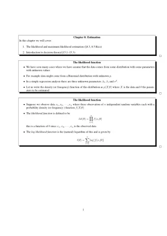
The likelihood function General considerations Definition of the likelihood function Data are a sequence of N observations, denoted y ∗ 1: N . A statistical model is a density function f Y 1: N ( y 1: N ; θ ) which defines a probability distribution for each value of a parameter vector θ . To perform statistical inference, we must decide, among other things, for which (if any) values of θ it is reasonable to model y ∗ 1: N as a random draw from f Y 1: N ( y 1: N ; θ ) . The likelihood function is L ( θ ) = f Y 1: N ( y ∗ 1: N ; θ ) , the density function evaluated at the data. It is often convenient to work with the log likelihood function, ℓ ( θ ) = log L ( θ ) = log f Y 1: N ( y ∗ 1: N ; θ ) . 8 / 74
The likelihood function General considerations Modeling using discrete and continuous distributions Recall that the probability distribution f Y 1: N ( y 1: N ; θ ) defines a random variable Y 1: N for which probabilities can be computed as integrals of f Y 1: N ( y 1: N ; θ ) . Specifically, for any event E describing a set of possible outcomes of Y 1: N , � P [ Y 1: N ∈ E ] = f Y 1: N ( y 1: N ; θ ) dy 1: N . E If the model corresponds to a discrete distribution, then the integral is replaced by a sum and the probability density function is called a probability mass function . The definition of the likelihood function remains unchanged. We will use the notation of continuous random variables, but all the methods apply also to discrete models. 9 / 74
The likelihood function General considerations A simulator is implicitly a statistical model For simple statistical models, we may describe the model by explicitly writing the density function f Y 1: N ( y 1: N ; θ ) . One may then ask how to simulate a random variable Y 1: N ∼ f Y 1: N ( y 1: N ; θ ) . For many dynamic models it is much more convenient to define the model via a procedure to simulate the random variable Y 1: N . This implicitly defines the corresponding density f Y 1: N ( y 1: N ; θ ) . For a complicated simulation procedure, it may be difficult or impossible to write down or even compute f Y 1: N ( y 1: N ; θ ) exactly. It is important to bear in mind that the likelihood function exists even when we don’t know what it is! We can still talk about the likelihood function, and develop numerical methods that take advantage of its statistical properties. 10 / 74
The likelihood function Likelihood of a POMP model The likelihood for a POMP model Recall the following schematic diagram, showing dependence among variables in a POMP model. Measurements, Y n , at time t n depend on the latent process, X n , at that time. The Markov property asserts that latent process variables depend on their value at the previous timestep. To be more precise, the distribution of the state X n +1 , conditional on X n , is independent of the values of X k , k < n and Y k , k ≤ n . Moreover, the distribution of the measurement Y n , conditional on X n , is independent of all other variables. 11 / 74
The likelihood function Likelihood of a POMP model The likelihood for a POMP model II 12 / 74
The likelihood function Likelihood of a POMP model The likelihood for a POMP model III The latent process X ( t ) may be defined at all times, but we are particularly interested in its value at observation times. Therefore, we write X n = X ( t n ) . We write collections of random variables using the notation X 0: N = ( X 0 , . . . , X N ) . The one-step transition density, f X n | X n − 1 ( x n | x n − 1 ; θ ) , together with the measurement density, f Y n | X n ( y n | x n ; θ ) and the initial density, f X 0 ( x 0 ; θ ) , specify the entire joint density via f X 0: N ,Y 1: N ( x 0: N , y 1: N ; θ ) N � = f X 0 ( x 0 ; θ ) f X n | X n − 1 ( x n | x n − 1 ; θ ) f Y n | X n ( y n | x n ; θ ) . n =1 13 / 74
The likelihood function Likelihood of a POMP model The likelihood for a POMP model IV The marginal density for sequence of measurements, Y 1: N , evaluated at the data, y ∗ 1: N , is � L ( θ ) = f Y 1: N ( y ∗ f X 0: N ,Y 1: N ( x 0: N , y ∗ 1: N ; θ ) = 1: N ; θ ) dx 0: N . 14 / 74
The likelihood function Likelihood of a POMP model Special case: deterministic latent process When the latent process is non-random, the log likelihood for a POMP model closely resembles a nonlinear regression model. In this case, we can write X n = x n ( θ ) , and the log likelihood is N � y ∗ � � ℓ ( θ ) = log f Y n | X n n | x n ( θ ); θ . n =1 If we have a Gaussian measurement model, where Y n given � � X n = x n ( θ ) is conditionally normal with mean ˆ y n x n ( θ ) and constant variance σ 2 , then the log likelihood contains a sum of squares which is exactly the criterion that nonlinear least squares regression seeks to minimize. More details on deterministic latent process models are given as a supplement. 15 / 74
The likelihood function Likelihood of a POMP model General case: stochastic unobserved state process For a POMP model, the likelihood takes the form of an integral: L ( θ ) = f Y 1: N ( y ∗ 1: N ; θ ) N � � f Y n | X n ( y ∗ = f X 0 ( x 0 ; θ ) n | x n ; θ ) f X n | X n − 1 ( x n | x n − 1 ; θ ) dx 0: N . n =1 (1) This integral is high dimensional and, except for the simplest cases, can not be reduced analytically. 16 / 74
Computing the likelihood Outline Introduction 1 The likelihood function 2 Likelihood of a POMP model Computing the likelihood 3 Sequential Monte Carlo Likelihood-based inference 4 Parameter estimates and uncertainty quantification Geometry of the likelihood function 5 Exercises 6 More on likelihood-based inference 7 Maximizing the likelihood Likelihood ratio test Information criteria 17 / 74
Computing the likelihood Monte Carlo algorithms Monte Carlo likelihood by direct simulation We work toward introducing the particle filter by first proposing a simpler method that usually doesn’t work on anything but very short time series. Although this section is a demonstration of what not to do , it serves as an introduction to the general approach of Monte Carlo integration. First, let’s rewrite the likelihood integral using an equivalent factorization. As an exercise, you could check how the equivalence of Eqns. 1 and 2 follows algebraically from the Markov property and the definition of conditional density. 18 / 74
Computing the likelihood Monte Carlo algorithms Monte Carlo likelihood by direct simulation II L ( θ ) = f Y 1: N ( y ∗ 1: N ; θ ) � � N � (2) � f Y n | X n ( y ∗ = n | x n ; θ ) f X 0: N ( x 0: N ; θ ) dx 0: N . n =1 Notice, using the representation in Eqn. 2, that the likelihood can be written as an expectation, � N � � f Y n | X n ( y ∗ L ( θ ) = E n | X n ; θ ) , n =1 where the expectation is taken with X 0: N ∼ f X 0: N ( x 0: N ; θ ) . 19 / 74
Recommend
More recommend
Explore More Topics
Stay informed with curated content and fresh updates.
