Learning a Belief Network If you know the structure have observed - PowerPoint PPT Presentation

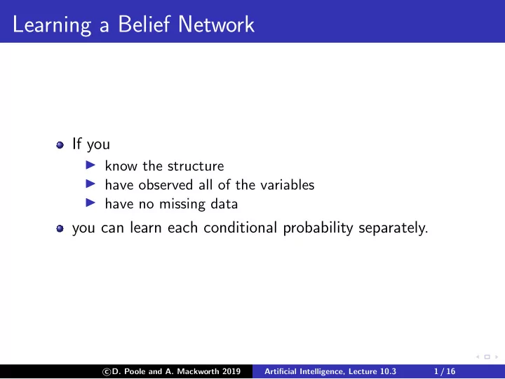
Learning a Belief Network If you ◮ know the structure ◮ have observed all of the variables ◮ have no missing data you can learn each conditional probability separately. � D. Poole and A. Mackworth 2019 c Artificial Intelligence, Lecture 10.3 1 / 16

Learning belief network example Model Data → Probabilities A B A B C D E P ( A ) t f t t f E P ( B ) f t t t t P ( E | A , B ) t t f t f C D P ( C | E ) · · · P ( D | E ) � D. Poole and A. Mackworth 2019 c Artificial Intelligence, Lecture 10.3 2 / 16

Learning conditional probabilities Each conditional probability distribution can be learned separately: For example: P ( E = t | A = t ∧ B = f ) (#examples: E = t ∧ A = t ∧ B = f ) + c 1 = (#examples: A = t ∧ B = f ) + c where c 1 and c reflect prior (expert) knowledge ( c 1 ≤ c ). When there are many parents to a node, there can little or no data for each conditional probability: � D. Poole and A. Mackworth 2019 c Artificial Intelligence, Lecture 10.3 3 / 16

Learning conditional probabilities Each conditional probability distribution can be learned separately: For example: P ( E = t | A = t ∧ B = f ) (#examples: E = t ∧ A = t ∧ B = f ) + c 1 = (#examples: A = t ∧ B = f ) + c where c 1 and c reflect prior (expert) knowledge ( c 1 ≤ c ). When there are many parents to a node, there can little or no data for each conditional probability: use supervised learning to learn a decision tree, linear classifier, a neural network or other representation of the conditional probability. � D. Poole and A. Mackworth 2019 c Artificial Intelligence, Lecture 10.3 3 / 16

Unobserved Variables A What if we had only observed values for A , B , C ? H A B C t f t f t t t t f B C · · · � D. Poole and A. Mackworth 2019 c Artificial Intelligence, Lecture 10.3 4 / 16

EM Algorithm Model Augmented Data Probabilities A B C H Count A t f t t 0 . 7 E-step P ( A ) 0 . 3 t f t f P ( H | A ) H f t t f 0 . 9 P ( B | H ) 0 . 1 f t t t P ( C | H ) · · · · · · M-step B C � D. Poole and A. Mackworth 2019 c Artificial Intelligence, Lecture 10.3 5 / 16

EM Algorithm Repeat the following two steps: ◮ E-step give the expected number of data points for the unobserved variables based on the given probability distribution. Requires probabilistic inference. � D. Poole and A. Mackworth 2019 c Artificial Intelligence, Lecture 10.3 6 / 16

EM Algorithm Repeat the following two steps: ◮ E-step give the expected number of data points for the unobserved variables based on the given probability distribution. Requires probabilistic inference. ◮ M-step infer the (maximum likelihood) probabilities from the data. This is the same as the fully-observable case. � D. Poole and A. Mackworth 2019 c Artificial Intelligence, Lecture 10.3 6 / 16

EM Algorithm Repeat the following two steps: ◮ E-step give the expected number of data points for the unobserved variables based on the given probability distribution. Requires probabilistic inference. ◮ M-step infer the (maximum likelihood) probabilities from the data. This is the same as the fully-observable case. Start either with made-up data or made-up probabilities. � D. Poole and A. Mackworth 2019 c Artificial Intelligence, Lecture 10.3 6 / 16

EM Algorithm Repeat the following two steps: ◮ E-step give the expected number of data points for the unobserved variables based on the given probability distribution. Requires probabilistic inference. ◮ M-step infer the (maximum likelihood) probabilities from the data. This is the same as the fully-observable case. Start either with made-up data or made-up probabilities. EM will converge to a local maxima. � D. Poole and A. Mackworth 2019 c Artificial Intelligence, Lecture 10.3 6 / 16

Belief network structure learning (I) Given examples e , and model m : P ( m | e ) = P ( e | m ) × P ( m ) P ( e ) . A model here is a belief network. � D. Poole and A. Mackworth 2019 c Artificial Intelligence, Lecture 10.3 7 / 16

Belief network structure learning (I) Given examples e , and model m : P ( m | e ) = P ( e | m ) × P ( m ) P ( e ) . A model here is a belief network. A bigger network can always fit the data better. � D. Poole and A. Mackworth 2019 c Artificial Intelligence, Lecture 10.3 7 / 16

Belief network structure learning (I) Given examples e , and model m : P ( m | e ) = P ( e | m ) × P ( m ) P ( e ) . A model here is a belief network. A bigger network can always fit the data better. P ( m ) lets us encode a preference for simpler models (e.g, smaller networks) � D. Poole and A. Mackworth 2019 c Artificial Intelligence, Lecture 10.3 7 / 16

Belief network structure learning (I) Given examples e , and model m : P ( m | e ) = P ( e | m ) × P ( m ) P ( e ) . A model here is a belief network. A bigger network can always fit the data better. P ( m ) lets us encode a preference for simpler models (e.g, smaller networks) − → search over network structure looking for the most likely model. � D. Poole and A. Mackworth 2019 c Artificial Intelligence, Lecture 10.3 7 / 16

A belief network structure learning algorithm Search over total orderings of variables. For each total ordering X 1 , . . . , X n use supervised learning to learn P ( X i | X 1 . . . X i − 1 ). Return the network model found with minimum: − log P ( e | m ) − log P ( m ) ◮ P ( e | m ) can be obtained by inference. ◮ How to determine − log P ( m )? � D. Poole and A. Mackworth 2019 c Artificial Intelligence, Lecture 10.3 8 / 16

Bayesian Information Criterion (BIC) Score P ( m | e ) = P ( e | m ) × P ( m ) P ( e ) − log P ( m | e ) ∝ − log P ( e | m ) − log P ( m ) � D. Poole and A. Mackworth 2019 c Artificial Intelligence, Lecture 10.3 9 / 16

Bayesian Information Criterion (BIC) Score P ( m | e ) = P ( e | m ) × P ( m ) P ( e ) − log P ( m | e ) ∝ − log P ( e | m ) − log P ( m ) − log P ( e | m ) is the negative log likelihood of model m : number of bits to describe the data in terms of the model. | e | is the number of examples. Each proposition can be true for between 0 and | e | examples, so there are different probabilities to distinguish. Each one can be described in bits. If there are || m || independent parameters ( || m || is the dimensionality of the model): − log P ( m | e ) ∝ � D. Poole and A. Mackworth 2019 c Artificial Intelligence, Lecture 10.3 9 / 16

Bayesian Information Criterion (BIC) Score P ( m | e ) = P ( e | m ) × P ( m ) P ( e ) − log P ( m | e ) ∝ − log P ( e | m ) − log P ( m ) − log P ( e | m ) is the negative log likelihood of model m : number of bits to describe the data in terms of the model. | e | is the number of examples. Each proposition can be true for between 0 and | e | examples, so there are | e | + 1 different probabilities to distinguish. Each one can be described in bits. If there are || m || independent parameters ( || m || is the dimensionality of the model): − log P ( m | e ) ∝ � D. Poole and A. Mackworth 2019 c Artificial Intelligence, Lecture 10.3 9 / 16

Bayesian Information Criterion (BIC) Score P ( m | e ) = P ( e | m ) × P ( m ) P ( e ) − log P ( m | e ) ∝ − log P ( e | m ) − log P ( m ) − log P ( e | m ) is the negative log likelihood of model m : number of bits to describe the data in terms of the model. | e | is the number of examples. Each proposition can be true for between 0 and | e | examples, so there are | e | + 1 different probabilities to distinguish. Each one can be described in log( | e | + 1) bits. If there are || m || independent parameters ( || m || is the dimensionality of the model): − log P ( m | e ) ∝ � D. Poole and A. Mackworth 2019 c Artificial Intelligence, Lecture 10.3 9 / 16

Bayesian Information Criterion (BIC) Score P ( m | e ) = P ( e | m ) × P ( m ) P ( e ) − log P ( m | e ) ∝ − log P ( e | m ) − log P ( m ) − log P ( e | m ) is the negative log likelihood of model m : number of bits to describe the data in terms of the model. | e | is the number of examples. Each proposition can be true for between 0 and | e | examples, so there are | e | + 1 different probabilities to distinguish. Each one can be described in log( | e | + 1) bits. If there are || m || independent parameters ( || m || is the dimensionality of the model): − log P ( m | e ) ∝ − log P ( e | m ) + || m || log( | e | + 1) This is (approximately) the BIC score. � D. Poole and A. Mackworth 2019 c Artificial Intelligence, Lecture 10.3 9 / 16

Belief network structure learning (II) Given a total ordering, to determine parents ( X i ) do independence tests to determine which features should be the parents � D. Poole and A. Mackworth 2019 c Artificial Intelligence, Lecture 10.3 10 / 16

Belief network structure learning (II) Given a total ordering, to determine parents ( X i ) do independence tests to determine which features should be the parents XOR problem: just because features do not give information individually, does not mean they will not give information in combination � D. Poole and A. Mackworth 2019 c Artificial Intelligence, Lecture 10.3 10 / 16