Belief network inference Four main approaches to determine posterior - PowerPoint PPT Presentation
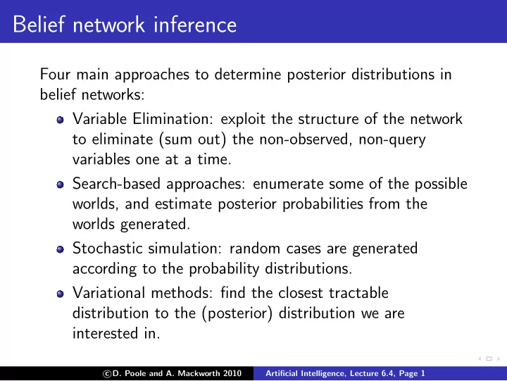
Belief network inference Four main approaches to determine posterior distributions in belief networks: Variable Elimination: exploit the structure of the network to eliminate (sum out) the non-observed, non-query variables one at a time.
Belief network inference Four main approaches to determine posterior distributions in belief networks: Variable Elimination: exploit the structure of the network to eliminate (sum out) the non-observed, non-query variables one at a time. Search-based approaches: enumerate some of the possible worlds, and estimate posterior probabilities from the worlds generated. Stochastic simulation: random cases are generated according to the probability distributions. Variational methods: find the closest tractable distribution to the (posterior) distribution we are interested in. � D. Poole and A. Mackworth 2010 c Artificial Intelligence, Lecture 6.4, Page 1
Factors A factor is a representation of a function from a tuple of random variables into a number. We will write factor f on variables X 1 , . . . , X j as f ( X 1 , . . . , X j ). We can assign some or all of the variables of a factor: f ( X 1 = v 1 , X 2 , . . . , X j ), where v 1 ∈ dom ( X 1 ), is a factor on X 2 , . . . , X j . f ( X 1 = v 1 , X 2 = v 2 , . . . , X j = v j ) is a number that is the value of f when each X i has value v i . The former is also written as f ( X 1 , X 2 , . . . , X j ) X 1 = v 1 , etc. � D. Poole and A. Mackworth 2010 c Artificial Intelligence, Lecture 6.4, Page 2
Example factors val Y Z X Y Z val t t 0.1 t t t 0.1 r ( X = t , Y , Z ): t f t t f 0.9 f t t f t 0.2 f f r ( X , Y , Z ): t f f 0.8 f t t 0.4 f t f 0.6 f f t 0.3 f f f 0.7 � D. Poole and A. Mackworth 2010 c Artificial Intelligence, Lecture 6.4, Page 3
Example factors val Y Z X Y Z val t t 0.1 t t t 0.1 r ( X = t , Y , Z ): t f 0.9 t t f 0.9 f t 0.2 t f t 0.2 f f 0.8 r ( X , Y , Z ): t f f 0.8 f t t 0.4 f t f 0.6 r ( X = t , Y , Z = f ): f f t 0.3 f f f 0.7 � D. Poole and A. Mackworth 2010 c Artificial Intelligence, Lecture 6.4, Page 4
Example factors val Y Z X Y Z val t t 0.1 t t t 0.1 r ( X = t , Y , Z ): t f t t f 0.9 f t t f t 0.2 f f r ( X , Y , Z ): t f f 0.8 f t t 0.4 Y val f t f 0.6 r ( X = t , Y , Z = f ): t f f t 0.3 f f f f 0.7 r ( X = t , Y = f , Z = f ) = � D. Poole and A. Mackworth 2010 c Artificial Intelligence, Lecture 6.4, Page 5
Example factors val Y Z X Y Z val t t 0.1 t t t 0.1 r ( X = t , Y , Z ): t f t t f 0.9 f t t f t 0.2 f f r ( X , Y , Z ): t f f 0.8 f t t 0.4 Y val f t f 0.6 r ( X = t , Y , Z = f ): t 0.9 f f t 0.3 f 0.8 f f f 0.7 r ( X = t , Y = f , Z = f ) = 0 . 8 � D. Poole and A. Mackworth 2010 c Artificial Intelligence, Lecture 6.4, Page 6
Multiplying factors The product of factor f 1 ( X , Y ) and f 2 ( Y , Z ), where Y are the variables in common, is the factor ( f 1 × f 2 )( X , Y , Z ) defined by: ( f 1 × f 2 )( X , Y , Z ) = f 1 ( X , Y ) f 2 ( Y , Z ) . � D. Poole and A. Mackworth 2010 c Artificial Intelligence, Lecture 6.4, Page 7
Multiplying factors example A B val t t 0.1 val A B C f 1 : t f 0.9 t t t 0.03 f t 0.2 t t f f f 0.8 t f t f 1 × f 2 : t f f B C val f t t t t 0.3 f t f f 2 : t f 0.7 f f t f t 0.6 f f f f f 0.4 � D. Poole and A. Mackworth 2010 c Artificial Intelligence, Lecture 6.4, Page 8
Multiplying factors example A B val t t 0.1 val A B C f 1 : t f 0.9 t t t 0.03 f t 0.2 t t f 0.07 f f 0.8 t f t 0.54 f 1 × f 2 : t f f 0.36 B C val f t t 0.06 t t 0.3 f t f 0.14 f 2 : t f 0.7 f f t 0.48 f t 0.6 f f f 0.32 f f 0.4 � D. Poole and A. Mackworth 2010 c Artificial Intelligence, Lecture 6.4, Page 9
Summing out variables We can sum out a variable, say X 1 with domain { v 1 , . . . , v k } , from factor f ( X 1 , . . . , X j ), resulting in a factor on X 2 , . . . , X j defined by: � ( f )( X 2 , . . . , X j ) X 1 = f ( X 1 = v 1 , . . . , X j ) + · · · + f ( X 1 = v k , . . . , X j ) � D. Poole and A. Mackworth 2010 c Artificial Intelligence, Lecture 6.4, Page 10
Summing out a variable example val A B C t t t 0.03 val t t f 0.07 A C t f t 0.54 t t 0.57 f 3 : t f f 0.36 � B f 3 : t f f t t 0.06 f t f t f 0.14 f f f f t 0.48 f f f 0.32 � D. Poole and A. Mackworth 2010 c Artificial Intelligence, Lecture 6.4, Page 11
Summing out a variable example val A B C t t t 0.03 val t t f 0.07 A C t f t 0.54 t t 0.57 f 3 : t f f 0.36 � B f 3 : t f 0.43 f t t 0.06 f t 0.54 f t f 0.14 f f 0.46 f f t 0.48 f f f 0.32 � D. Poole and A. Mackworth 2010 c Artificial Intelligence, Lecture 6.4, Page 12
Exercise Given factors: val A B A val t t 0.6 A val s: t 0.75 t: t f 0.4 o: t 0.3 f 0.25 f t 0.2 f 0.1 f f 0.8 What is? (a) s × t (b) � A s × t (c) � B s × t (d) s × t × o (e) � A s × t × o (f) � b s × t × o � D. Poole and A. Mackworth 2010 c Artificial Intelligence, Lecture 6.4, Page 13
Evidence If we want to compute the posterior probability of Z given evidence Y 1 = v 1 ∧ . . . ∧ Y j = v j : P ( Z | Y 1 = v 1 , . . . , Y j = v j ) = � D. Poole and A. Mackworth 2010 c Artificial Intelligence, Lecture 6.4, Page 14
Evidence If we want to compute the posterior probability of Z given evidence Y 1 = v 1 ∧ . . . ∧ Y j = v j : P ( Z | Y 1 = v 1 , . . . , Y j = v j ) P ( Z , Y 1 = v 1 , . . . , Y j = v j ) = P ( Y 1 = v 1 , . . . , Y j = v j ) = � D. Poole and A. Mackworth 2010 c Artificial Intelligence, Lecture 6.4, Page 15
Evidence If we want to compute the posterior probability of Z given evidence Y 1 = v 1 ∧ . . . ∧ Y j = v j : P ( Z | Y 1 = v 1 , . . . , Y j = v j ) P ( Z , Y 1 = v 1 , . . . , Y j = v j ) = P ( Y 1 = v 1 , . . . , Y j = v j ) P ( Z , Y 1 = v 1 , . . . , Y j = v j ) = � Z P ( Z , Y 1 = v 1 , . . . , Y j = v j ) . So the computation reduces to the probability of P ( Z , Y 1 = v 1 , . . . , Y j = v j ). We normalize at the end. � D. Poole and A. Mackworth 2010 c Artificial Intelligence, Lecture 6.4, Page 16
Probability of a conjunction Suppose the variables of the belief network are X 1 , . . . , X n . To compute P ( Z , Y 1 = v 1 , . . . , Y j = v j ), we sum out the other variables, Z 1 , . . . , Z k = { X 1 , . . . , X n } − { Z } − { Y 1 , . . . , Y j } . We order the Z i into an elimination ordering. P ( Z , Y 1 = v 1 , . . . , Y j = v j ) = � D. Poole and A. Mackworth 2010 c Artificial Intelligence, Lecture 6.4, Page 17
Probability of a conjunction Suppose the variables of the belief network are X 1 , . . . , X n . To compute P ( Z , Y 1 = v 1 , . . . , Y j = v j ), we sum out the other variables, Z 1 , . . . , Z k = { X 1 , . . . , X n } − { Z } − { Y 1 , . . . , Y j } . We order the Z i into an elimination ordering. P ( Z , Y 1 = v 1 , . . . , Y j = v j ) � � = · · · P ( X 1 , . . . , X n ) Y 1 = v 1 ,..., Y j = v j . Z k Z 1 = � D. Poole and A. Mackworth 2010 c Artificial Intelligence, Lecture 6.4, Page 18
Probability of a conjunction Suppose the variables of the belief network are X 1 , . . . , X n . To compute P ( Z , Y 1 = v 1 , . . . , Y j = v j ), we sum out the other variables, Z 1 , . . . , Z k = { X 1 , . . . , X n } − { Z } − { Y 1 , . . . , Y j } . We order the Z i into an elimination ordering. P ( Z , Y 1 = v 1 , . . . , Y j = v j ) � � = · · · P ( X 1 , . . . , X n ) Y 1 = v 1 ,..., Y j = v j . Z k Z 1 n � � � = · · · P ( X i | parents ( X i )) Y 1 = v 1 ,..., Y j = v j . Z k Z 1 i =1 � D. Poole and A. Mackworth 2010 c Artificial Intelligence, Lecture 6.4, Page 19
Computing sums of products Computation in belief networks reduces to computing the sums of products. How can we compute ab + ac efficiently? � D. Poole and A. Mackworth 2010 c Artificial Intelligence, Lecture 6.4, Page 20
Computing sums of products Computation in belief networks reduces to computing the sums of products. How can we compute ab + ac efficiently? Distribute out the a giving a ( b + c ) � D. Poole and A. Mackworth 2010 c Artificial Intelligence, Lecture 6.4, Page 21
Computing sums of products Computation in belief networks reduces to computing the sums of products. How can we compute ab + ac efficiently? Distribute out the a giving a ( b + c ) � n How can we compute � i =1 P ( X i | parents ( X i )) Z 1 efficiently? � D. Poole and A. Mackworth 2010 c Artificial Intelligence, Lecture 6.4, Page 22
Computing sums of products Computation in belief networks reduces to computing the sums of products. How can we compute ab + ac efficiently? Distribute out the a giving a ( b + c ) � n How can we compute � i =1 P ( X i | parents ( X i )) Z 1 efficiently? Distribute out those factors that don’t involve Z 1 . � D. Poole and A. Mackworth 2010 c Artificial Intelligence, Lecture 6.4, Page 23
Variable elimination algorithm To compute P ( Z | Y 1 = v 1 ∧ . . . ∧ Y j = v j ): Construct a factor for each conditional probability. Set the observed variables to their observed values. Sum out each of the other variables (the { Z 1 , . . . , Z k } ) according to some elimination ordering. Multiply the remaining factors. Normalize by dividing the resulting factor f ( Z ) by � Z f ( Z ). � D. Poole and A. Mackworth 2010 c Artificial Intelligence, Lecture 6.4, Page 24
Recommend
More recommend
Explore More Topics
Stay informed with curated content and fresh updates.





![Bayesian Belief Networks Decision Theoretic Agents Introduction to Probability [Ch13]](https://c.sambuz.com/890744/bayesian-belief-networks-decision-theoretic-agents-s.webp)
