Likelihood inference in complex settings Nancy Reid with Uyen - PowerPoint PPT Presentation
Likelihood inference for simple problems Higher order approximation Harder problems Approximations to likelihoods Likelihood inference in complex settings Nancy Reid with Uyen Hoang, Wei Lin, Ximing Xu 1 / 30 Likelihood inference for simple
Likelihood inference for simple problems Higher order approximation Harder problems Approximations to likelihoods Likelihood inference in complex settings Nancy Reid with Uyen Hoang, Wei Lin, Ximing Xu 1 / 30
Likelihood inference for simple problems Higher order approximation Harder problems Approximations to likelihoods Likelihood inference for simple problems Higher order approximation Harder problems Approximations to likelihoods 2 / 30
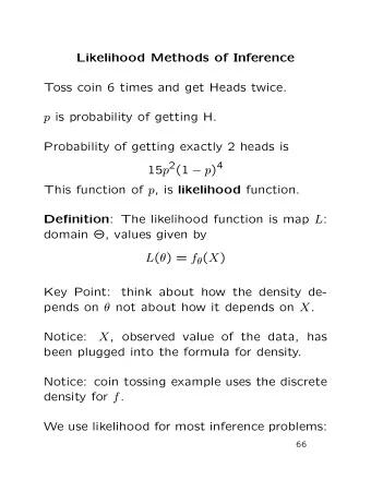
Likelihood inference for simple problems Higher order approximation Harder problems Approximations to likelihoods Why likelihood? • likelihood function depends on data only through sufficient statistics • “likelihood map is sufficient” Fraser & Naderi, 2006 • provides summary statistics with known limiting distribution • leading to approximate pivotal functions, based on normal distribution • in some models the likelihood function gives exact inference • “likelihood function as pivotal” Hinkley, 1980 • likelihood function + sample space derivative gives better approximate inference 3 / 30
Likelihood inference for simple problems Higher order approximation Harder problems Approximations to likelihoods Summary statistics and approximate pivotals f ( y ; θ ) , y ∈ R n , θ ∈ R d • model • log-likelihood function ℓ ( θ ; y ) = log f ( y ; θ ) + a ( y ) • score function u ( θ ) = ∂ℓ ( θ ; y ) /∂θ ˆ • maximum likelihood estimate θ = arg sup θ ℓ ( θ ; y ) w ( θ ) = 2 { ℓ (ˆ • log-likelihood ratio θ ; y ) − ℓ ( θ ; y ) } 4 / 30
Likelihood inference for simple problems Higher order approximation Harder problems Approximations to likelihoods Approximate pivotals √ n (ˆ θ − θ ) . ∼ N d { 0 , j − 1 (ˆ θ ) } θ ) − ℓ ( θ ) } . w ( θ ) = 2 { ℓ (ˆ ∼ χ 2 d 1 √ nU ( θ ) . ∼ N d { 0 , j (ˆ θ ) } 1 L √ nU ( θ ) − → N d { 0 , I ( θ ) } j (ˆ θ ) = − ℓ ′′ (ˆ θ ) / n I ( θ ) = E { j ( θ ) } 5 / 30
Likelihood inference for simple problems Higher order approximation Harder problems Approximations to likelihoods ...approximate pivotals log−likelihood function 0 −1 log−likelihood −2 −3 −4 16 17 18 19 20 21 22 23 θ 6 / 30
Likelihood inference for simple problems Higher order approximation Harder problems Approximations to likelihoods ...approximate pivotals log−likelihood function 0 −1 log−likelihood −2 −3 −4 θ 16 17 18 19 20 21 22 23 θ 7 / 30
Likelihood inference for simple problems Higher order approximation Harder problems Approximations to likelihoods ...approximate pivotals log−likelihood function 0 −1 log−likelihood −2 θ − θ −3 −4 θ 16 17 18 19 20 21 22 23 θ 8 / 30
Likelihood inference for simple problems Higher order approximation Harder problems Approximations to likelihoods ...approximate pivotals log−likelihood function 0 −1 log−likelihood −2 θ − θ −3 −4 θ 16 17 18 19 20 21 22 23 θ 9 / 30
Likelihood inference for simple problems Higher order approximation Harder problems Approximations to likelihoods ...approximate pivotals log−likelihood function 0 −1 1.92 w/2 log−likelihood −2 θ − θ −3 −4 θ 16 17 18 19 20 21 22 23 θ 10 / 30
Likelihood inference for simple problems Higher order approximation Harder problems Approximations to likelihoods ...approximate pivotals θ ) − ℓ ( θ ) } . w ( θ ) = 2 { ℓ (ˆ ∼ χ 2 d M M (a) (a) -3 -2 -2 M -3 M -3 M M -4 M -4 -4 m -2 M 0 M 1 M 2 M 2 M 1 M M -1 0 M M M -1 M -1 2 M 2 M -3 -3 M -3 M -4 -2 -2 M M -2 M -1 -1 -4 M 1 M 1 M M 0 m 0 -4 M -1 (a) 2 1 0 -1 -2 -3 -4 -4 -3 -2 -1 0 1 2 11 / 30
Likelihood inference for simple problems Higher order approximation Harder problems Approximations to likelihoods Likelihood as pivotal • Example: location model f ( y ; θ ) = � n i = 1 f 0 ( y i − θ ) , θ ∈ R exp { ℓ ( θ ; y ) } f (ˆ • Fisher (1934) θ | a ; θ ) = � exp { ℓ ( θ ; y ) } d θ • → (ˆ a i = y i − ˆ ( y 1 , . . . , y n ) ← θ, a 1 , . . . , a n ) θ • exact (conditional) distribution of maximum likelihood estimator given by renormalized likelihood function • p ∗ approximation: θ ) | 1 / 2 exp { ℓ ( θ ; ˆ p ∗ (ˆ θ | a ; θ ) = c ( θ, a ) | j (ˆ θ, a ) − ℓ (ˆ θ ; ˆ θ, a ) } 12 / 30
Likelihood inference for simple problems Higher order approximation Harder problems Approximations to likelihoods A simpler approach • avoid → (ˆ ( y 1 , . . . , y n ) ← θ, a ) • define a derivative ∂ � ϕ ( θ ) ≡ ℓ ; V ( θ ; y 0 ) = � ∂ V ( y ) ℓ ( θ ; y ) � � y = y 0 • a directional derivative on the sample space • along with ℓ ( θ ; y 0 ) the observed log-likelihood function • can be extended to derivative of mean likelihood – usable in wider context Fraser/R Bka 2009 13 / 30
Likelihood inference for simple problems Higher order approximation Harder problems Approximations to likelihoods Tangent exponential model • A continuous model f ( y ; θ ) on R n can be approximated by an exponential family model on R d : f TEM ( s ; θ ) ds = exp { ϕ ( θ ) ′ s + ℓ 0 ( θ ) } h ( s ) ds (1) s ( y ) = − ℓ ϕ (ˆ • s is a score variable on R d θ 0 ; y ) • ℓ 0 ( θ ) = ℓ ( θ ; y 0 ) is the observed log-likelihood function • ϕ ( θ ) = ϕ ( θ ; y 0 ) is the directional derivative ℓ ; V ( θ ; y 0 ) • (1) approximates original model to O ( n − 1 ) • gives approximation to the p -value for testing θ • p -value is accurate to O ( n − 3 / 2 ) 14 / 30
Cauchy density and TEM approximation 0.30 0.25 0.20 density 0.15 0.10 0.05 -4 -2 0 2 4 y
Likelihood inference for simple problems Higher order approximation Harder problems Approximations to likelihoods Example: microscopic fluorescence • “tracking of microscopic fluorescent particles attached to biological specimens” Hughes et al., AOAS, 2010 • “CCD (charge-coupled device) camera attached to a microscope used to observe the specimens repeatedly” • “we introduce an improved technique for analyzing such images over time” • Model for counts: − ( x i − x j ) 2 + ( y i − y j ) 2 � � � Z i ∼ N ( f i , f i + ψ ) , f i ≃ B + A j exp S 2 j • f i developed from a model for photon emission; Normal approximation to Poisson; ψ catches the instrument error 16 / 30
Likelihood inference for simple problems Higher order approximation Harder problems Approximations to likelihoods ... microscopic fluorescence • “Our method, which applies maximum likelihood principles, improves the fit to the data, derives accurate standard errors from the data with minimal computation, and uses model-selection criteria to “count” the fluorophores in an image” • “likelihood ratio tests are used to select the final model” • potential for improved inference using likelihood methods? 17 / 30
Likelihood inference for simple problems Higher order approximation Harder problems Approximations to likelihoods ... a simpler model Y i ∼ N ( µ i , µ i + ψ ) , µ i = exp ( β 0 + β 1 x i ) approximate pivot r ∗ constructed from ℓ ( θ ; y 0 ) , ϕ ( θ ; y 0 ) should follow a N ( 0 , 1 ) distribution – simulations Normal Q-Q Plot 3 2 Sample Quantiles 1 0 -1 -2 -3 18 / 30 -3 -2 -1 0 1 2 3
Likelihood inference for simple problems Higher order approximation Harder problems Approximations to likelihoods More realistic models • for example for analytic inferences for survey data • stochastic processes in space or space-time • extremes in several dimensions • frailty models in survival data • longitudinal data • family-based genetic data and other forms of clustering • estimation of recombination rates from SNP data • ... 19 / 30
Likelihood inference for simple problems Higher order approximation Harder problems Approximations to likelihoods Example: Gaussian random field • scalar output y at p − dimensional input x = ( x 1 , . . . , x p ) • y ( x ) = φ ( x ) T β + Z ( x ) , Z ( x ) Gaussian process on R p • p Cov { Z ( x 1 ) , Z ( x 2 ) } = σ 2 � R ( | x 1 i − x 2 i | ; θ ) i = 1 • R ( | x 1 i − x 2 i | ) = exp {− γ i | x 1 i − x 2 i | α } • anisotropic covariance matrix for inputs on different scales • application to computer experiments Ximing Xu,U Toronto; Derek Bingham, SFU 20 / 30
Likelihood inference for simple problems Higher order approximation Harder problems Approximations to likelihoods ... Gaussian random field y n = ( y 1 , . . . , y n ) = { y ( x 1 ) , . . . , y ( x n ) } , at n locations x i in R p ℓ ( β, σ, θ ) = − 1 2 { n log σ 2 + log | R ( θ ) | + 1 σ 2 ( y n − Φ β ) T R − 1 ( θ )( y n − Φ β ) } , computation of R − 1 is O ( n 3 ) , n typically 100s or 1000s solution – make the correlation matrix sparse solution – simplify the likelihood function 21 / 30
Recommend
More recommend
Explore More Topics
Stay informed with curated content and fresh updates.
