STAT 339 A Generative Linear Model and Max Likelihood Estimation - PowerPoint PPT Presentation
STAT 339 A Generative Linear Model and Max Likelihood Estimation 20-22 February 2017 Colin Reimer Dawson 1 / 23 Questions/Administrative Business? 2 / 23 Outline Linear Model Revisited Maximum Likelihood Estimation 3 / 23 Linear Model
STAT 339 A Generative Linear Model and Max Likelihood Estimation 20-22 February 2017 Colin Reimer Dawson 1 / 23
Questions/Administrative Business? 2 / 23
Outline Linear Model Revisited Maximum Likelihood Estimation 3 / 23
Linear Model Revisited Our original formulation of the model was deterministic : for a given x , the model yields the same t every time. 5 / 23
Modeling the “Errors” Of course, the actual data is more complicated. 6 / 23
Adding Error to the Model ▸ We can capture this added complexity with a “catchall” error term, ε . t = w 0 + w 1 x 1 + ⋅⋅⋅ + w k x k + ε (1) ▸ ε is different for every case, even if x is the same. ▸ It is a different beast from the variables x , w and t : it is a random variable . ▸ A stand in for all the factors that we are not modeling. 7 / 23
A Generative Linear Model If each observation is associated with a random ε n term, then we have a generative model : t n = w 0 + w 1 x n 1 + ⋅⋅⋅ + w D x nD + ε n = x n w + ε n where ε i is a random error term. 8 / 23
More specifically... The classic case is when t n = x i w + ε n where the ε i are independent and identically distributed as N( 0 ,σ 2 ) random variables. 9 / 23
The Likelihood Function Previously, we chose ˆ w so as to minimize a loss function. With a generative model, an alternative is to find the parameters that make the data maximally likely . The Likelihood Function If the distribution of a r.v. X (or a random vector x ) depends on a parameter vector θ , then given an observation X = x (or x = x 0 ), the likelihood function is the probability (or density) of x (or x 0 ) for each possible value of θ : L ( θ ; x 0 ) = p ( x 0 ; θ ) 11 / 23
Example: Poisson Distribution The Poisson distribution with parameter λ is a discrete distribution on { 0 , 1 , 2 ,..., } with PMF p ( y ; λ ) = e − λ λ y y ! The likelihood function for λ is also L ( λ ; y ) = e − λ λ y y ! but considered as a function of λ for fixed observation y . 12 / 23
Poisson PMF and Likelihood 0.30 0.20 0.15 0.20 L ( λ ) p(y) 0.10 0.10 0.05 0.00 0.00 0 2 4 6 8 10 0 2 4 6 8 10 λ y Figure: Left: PMF for y from a Poisson ( λ ) distribution with λ = 1 . 5 . Right: Likelihood function for λ for a Poisson ( λ ) distribution with y = 3 . 13 / 23
Maximizing the Likelihood A reasonable criterion for estimating a parameter is to try to maximize the likelihood; i.e., choose the param that makes the data as “probable” as possible. MLE ˆ θ = arg max L ( θ ; x ) = arg max p ( x ; θ ) θ θ 14 / 23
Poisson MLE 0.30 0.20 0.15 0.20 p(y) L ( λ ) 0.10 0.10 0.05 0.00 0.00 0 2 4 6 8 10 0 2 4 6 8 10 λ y Figure: Left: PMF for y from a Poisson ( λ ) distribution with λ = 1 . 5 . Right: Likelihood function for λ for a Poisson ( λ ) distribution with y = 3 . What is the MLE for λ ? 15 / 23
Analytically... L ( λ ; y ) = e − λ λ y y ! dL ( λ ) = 1 y ! ( ye − λ λ y − 1 − e − λ λ y ) dλ Set to zero and solve.... λ y − 1 = e − ˆ ye − ˆ λ ˆ λ ˆ λ y ˆ λ = y 16 / 23
Log Likelihoods Many many common likelihoods are more manageable after taking a log. Also, if we have several independent observations, likelihoods multiply, but log likelihoods add. Can we just maximize the log likelihood instead? log L ( λ ; y ) = − λ + y log ( λ ) − log ( y ! ) d log L ( λ ) = − 1 + y dλ λ ˆ λ = y 17 / 23
Deriving the Likelihood Function for w The classic case is when t n = x i w + ε n where the ε i are independent and identically distributed as N( 0 ,σ 2 ) random variables. 18 / 23
Family of Conditional Densities for t n ε n ∼ N( 0 ,σ 2 ) ⇒ t n ∣ x n w ∼ N( x n w ,σ 2 ) − 1 / 2 exp {− 1 2 σ 2 ( t n − x n w ) 2 } i.e. p ( t n ∣ x n , w ,σ 2 ) = ( 2 πσ 2 ) 19 / 23
Family of Joint Densities for t Since we assume the ε n are independent, then after fixing (i.e., conditioning on) x n w for each n , the t n are also (conditionally) independent: N p ( t ∣ X , w ,σ 2 ) = ∏ p ( t n ∣ x n , w ,σ 2 ) n = 1 N − 1 / 2 exp { − 1 2 σ 2 ( t n − x n w ) 2 } = ( 2 πσ 2 ) ∏ n = 1 N − N / 2 exp { − 1 ( t n − x n w ) 2 } = ( 2 πσ 2 ) ∑ 2 σ 2 n = 1 − N / 2 exp { − 1 = ( 2 πσ 2 ) 2 σ 2 ( t − Xw ) T ( t − Xw )} 20 / 23
Finding the MLE for w − N / 2 exp { − 1 L ( w ,σ 2 ; X , t ) = ( 2 πσ 2 ) 2 σ 2 ( t − Xw ) T ( t − Xw )} Taking the log to make finding the gradient (much!) easier... log L ( w ,σ 2 ; X , t ) = − N 2 log ( 2 πσ 2 ) − 1 2 σ 2 ( t − Xw ) T ( t − Xw ) Taking the gradient w.r.t w ... ∂ log L ( w ,σ 2 ; X , t ) = 1 σ 2 X T ( t − Xw ) ∂ w and setting to zero... − 1 X T t w = X T t ⇒ w = ( X T X ) X T Xˆ ˆ 21 / 23
Finding the MLE for σ 2 If we want our estimated model to be generative, we also need to estimate σ 2 . log L ( w ,σ 2 ; X , t ) = − N 2 log ( 2 πσ 2 ) − 1 2 σ 2 ( t − Xw ) T ( t − Xw ) Taking the derivative w.r.t σ 2 ... ∂ log L ( w ,σ 2 ; X , t ) = − N 1 2 σ 2 + 2 ( σ 2 ) 2 ( t − Xw ) T ( t − Xw ) ∂σ 2 and setting to zero... σ 2 = 1 N ( t − Xw ) T ( t − Xw ) ˆ N = 1 2 ( t n − ˆ t n ) ∑ N n = 1 22 / 23
Summary: MLE Linear Regression Having defined a generative model according to ind. t n = x n w + ε n , ∼ N( 0 ,σ 2 ) ε n we get MLEs for w and σ 2 given by: − 1 X T t w = ( X T X ) ˆ σ 2 = 1 N ( t n − x n ˆ w ) 2 ˆ 23 / 23
Recommend
More recommend
Explore More Topics
Stay informed with curated content and fresh updates.
