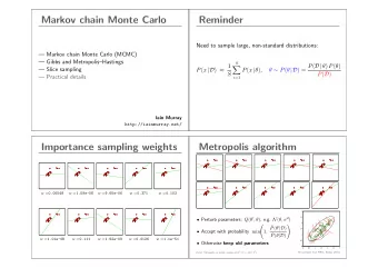
STAT 339 Markov Chain Monte Carlo (MCMC) 7 April 2017 Some theory - PowerPoint PPT Presentation

STAT 339 Markov Chain Monte Carlo (MCMC) 7 April 2017 Some theory and intuition about MCMC generally

Outline Gibbs Sampling in Mixture Models Sampling as an Approximation Method Gibbs Sampling Intuition and Motivation Concretely: The Algorithm A Bit of MCMC Theory

Outline Gibbs Sampling in Mixture Models Sampling as an Approximation Method Gibbs Sampling Intuition and Motivation Concretely: The Algorithm A Bit of MCMC Theory 3 / 31

Outline Gibbs Sampling in Mixture Models Sampling as an Approximation Method Gibbs Sampling Intuition and Motivation Concretely: The Algorithm A Bit of MCMC Theory 4 / 31

Intractable Posterior ▸ It is easy to write down the unnormalized posterior density: p ( θ ∣ Y ) ∝ p ( θ ) p ( Y ∣ θ ) ▸ GMM case: ( π k N( y n ∣ µ k , Σ k )) K N K p ( θ ∣ Y ) ∝ p ( π ) p ( µ k , Σ k ) ∏ ∏ ∑ k = 1 n = 1 k = 1 where, e.g., p ( π ) is Dirichlet, p ( µ k , Σ k ) is Normal-Inverse Wishart (or p ( µ k , Σ − 1 k ) is Normal-Wishart) ▸ But hard to do much with it (except maybe find a local maximum) ▸ Solution: Try to draw samples from it. 5 / 31

When can we sample from but not analyze a distribution? ▸ Consider trying to evaluate P ( Straight ) in poker (say) ▸ You might be able to do this analytically, but if you have a computer handy, it is easy to simulate dealing out several million poker hands ▸ Then, simply count: P ( Straight ) ≈ 1 S I ( Did I get a straight in hand s? ) ∑ S s = 1 6 / 31

Outline Gibbs Sampling in Mixture Models Sampling as an Approximation Method Gibbs Sampling Intuition and Motivation Concretely: The Algorithm A Bit of MCMC Theory 7 / 31

Gibbs Sampling as "Stochastic EM" ▸ The EM algorithm involves, iteratively 1. Computing an expectation over cluster assignments (using the posterior, conditioned on parameter values) 2. Arg-Maximizing parameter values (using the likelihood/posterior conditioned on expected cluster assignments) ▸ Gibbs sampling (in this context) involves, iteratively 1. Sampling cluster assignments (using the posterior, conditioned on parameter values) 2. Sampling parameter values (using the posterior, conditioned on cluster assignments) 8 / 31

What does Gibbs Yield? ▸ Over many iterations, Gibbs sampling yields a collection of many cluster assignments and many parameter values, distributed according to the joint posterior {{ z ( s ) n } N n = 1 , π ( s ) , { µ ( s ) k } K k = 1 }} S k , Σ ( s ) s = 1 ▸ These can be used to approximate more or less any function of the assignments and parameters we want ▸ Example: p ( z n = z m ∣ Y ) ≈ 1 S I ( z ( s ) = z ( s ) m ) ∑ n S s = 1 ▸ Or, for future data: m N( y new ∣ µ z ( s ) m ) π ( s ) ∑ m , Σ z ( s ) S p ( z new = z m ∣ y new , Y ) ≈ 1 z ( s ) k N( y new ∣ µ ( s ) k ) ∑ K k = 1 π ( s ) k , Σ ( s ) S s = 1 9 / 31

Outline Gibbs Sampling in Mixture Models Sampling as an Approximation Method Gibbs Sampling Intuition and Motivation Concretely: The Algorithm A Bit of MCMC Theory 10 / 31

Concretely: The Algorithm ▸ In general, Gibbs sampling applies when we have multiple sets of unknown parameters, but where it is difficult to sample all of them directly from their joint distribution. ▸ Mixture model: params are z , π and θ ▸ Idea: partition the parameters into “blocks”, and iteratively fix all but one block and sample the remaining from its posterior conditioned on the others ▸ Here, we need 1: p ( z ∣ Y , θ , π ) 2: p ( θ , π ∣ z , Y ) 11 / 31

Summary: Gibbs Algorithm for GMM 1. Initialize cluster assignments, z ( 0 ) (e.g., using K -means) 2. For s = 1 ,...,S , sample ∼ p ( µ k , Σ k ∣ z ( s − 1 ) , Y ) ,k = 1 ,...,K (a) µ ( s ) k , Σ ( s ) k (or, alternatively, subdivide into two blocks with µ k and Σ k sampled separately given the other) (b) π ( s ) ∼ p ( π ∣ z ( s − 1 ) ) ∼ p ( z n ∣ π ( s ) , θ ( s ) , y n ) ,n = 1 ,...,N (c) z ( s ) n 12 / 31

Specific Conditional Distributions Assuming conjugate priors and Σ k restricted to diagonal w/ elements h k,d = σ 2 k,d p ( µ k,d ∣ h k,d , z , Y ) = N( µ post ,h − 1 post ) where µ post = h − 1 post ( h prior µ prior + n k h k,d ¯ y k,d ) h post = h prior + n k h k,d p ( h k,d ∣ µ k , z , Y ) = Gamma ( a post ,b post ) where a post = a prior + n k 2 b post = b prior + 1 ( y n,d − µ k,d ) 2 2 ∑ n ∶ z n = k p ( π ∣ z , Y ) = Dir ( α post, 1 ,...,α post,K ) where α post,k = α prior,k + n k Each of these can be sampled from with readily available methods (e.g., numpy.random.dirichlet() ) 13 / 31

Conditional for z We have already worked out that p ( z n = k ∣ π , θ , Y ) = Categorical ( q n 1 ,...,q nK ) π k N( y n ∣ µ k , Σ k ) where q nk = k ′ = 1 π k N( y n ∣ µ k , Σ k ) ∑ K Conditioned on the cluster parameters, all z n are independent. Sampling from this distribution is just a matter of enumerating the probabilities, or using a library function for categorical distributions (e.g., numpy.random.choice() ) 14 / 31

Gibbs Sampling More Generally ▸ Gibbs is a very general algorithm that can be used to sample from complicated probability distributions ▸ In general suppose we have p ( θ ) = p ( θ 1 ,..., θ M ) where each θ m is a collection of random variables. We can generate samples from this distribution by 1. Initializing each θ m 2. For s = 1 ,...,S ; For m = 1 ,...,M : m from p ( θ m ∣ θ ( s ) ) 1 ,..., θ ( s ) m − 1 , θ ( s − 1 ) m + 1 ,..., θ ( s − 1 ) Sample θ ( s ) M ▸ Note that we can partition θ into the θ m however we like, as long as certain conditions are met (more on this later) 15 / 31

Application: Image De-Noising Consider a generative model of noisy images in which θ represents the pixels of the “pure” image, and Y is the observed “corrupted” image. 16 / 31

Application: Image De-Noising ▸ We can define a prior on θ that encourages neighboring pixels to be similar, and a likelihood on Y that encourages observed pixels to be close to the corresponding one in the pure image. ▸ Then, we Gibbs sample each pixel θ m conditioned on the image and the other θ s p ( θ m ∣ θ − m , Y ) ∝ p ( θ m ∣ θ m − ) p ( y m ∣ θ m ) 17 / 31

Results from Two Priors 18 / 31

Outline Gibbs Sampling in Mixture Models Sampling as an Approximation Method Gibbs Sampling Intuition and Motivation Concretely: The Algorithm A Bit of MCMC Theory 19 / 31

Markov Chain Monte Carlo ▸ MCMC gets its name from the fact that it is a method for generating random samples (the “Monte Carlo” part) and the fact that each sample depends on exactly one previous sample (the “Markov Chain”) part ▸ In general, involves sampling from q ( θ ( s ) ∣ θ ( s − 1 ) ) for a suitable “transition kernel” q . ▸ Under certain conditions, θ ( s for large s are distributed according to p ( θ ) , which is determined by q . ▸ Idea: construct a q so that p is the target distribution we want to get samples from. 20 / 31

Markov Chains ▸ Simple Markov chain: two possible states, { rain,sun } at each time step t . ▸ Suppose q ( ⋅ ∣ ⋅ ) is defined by the transition matrix ⎛ ⎞ rain sun Q = ⎜ ⎟ rain 0 . 7 0 . 3 ⎝ ⎠ sun 0 . 1 0 . 9 where rows represent the “from” state and columns represent the “to” state. That is, q ( rain ∣ rain ) = 0 . 7 , q ( sun ∣ rain ) = 0 . 3 , etc. 21 / 31

Markov Chains ▸ Suppose q ( ⋅ ∣ ⋅ ) is defined by the transition matrix ⎛ ⎞ rain sun ⎜ ⎟ Q = rain 0 . 7 0 . 3 ⎝ ⎠ sun 0 . 1 0 . 9 ▸ Question: If it is sunny today, what is the probability that it will be sunny tomorrow? ▸ If it is sunny today, what is the probability that it will be rainy two days from now? 22 / 31

Markov Chains ▸ Suppose q ( ⋅ ∣ ⋅ ) is defined by the transition matrix ⎛ ⎞ rain sun Q = ⎜ ⎟ rain 0 . 7 0 . 3 ⎝ ⎠ sun 0 . 1 0 . 9 ▸ If it is sunny today, what is the probability that it will be rainy two days from now? ▸ We have P ( θ t + 2 = rain ∣ θ t = sun ) = ∑ P ( θ t + 1 = s,θ t + 2 = rain ∣ θ t = sun ) s = ∑ q ( s ∣ sun ) q ( rain ∣ s ) s = ( QQ ) 2 , 2 = ( 0 . 1 , 0 . 9 ) T ( 0 . 7 , 0 . 1 ) = 0 . 07 + 0 . 09 = 0 . 16 23 / 31

Markov Chains ▸ Suppose q ( ⋅ ∣ ⋅ ) is defined by the transition matrix ⎛ ⎞ rain sun Q = ⎜ ⎟ rain 0 . 7 0 . 3 ⎝ ⎠ sun 0 . 1 0 . 9 ▸ If it is sunny today, what is the probability that it will be rainy a year from now? ▸ We have the recurrence relation P ( θ t + m ∣ θ t ) = ∑ P ( θ t + m − 1 = s,θ t + m ∣ θ t ) s ▸ This is the matrix product of the m − 1 step matrix with the one-step transition matrix. ▸ So the m -step transition matrix is just Q m 24 / 31

Simulation of Q ∞ ▸ What does the “many step” transition matrix look like? ▸ Simulation ▸ We find that regardless of the starting state, there is a 1/4 chance of rain and a 3/4 chance of sun on any day far enough in the future. ▸ This is called the stationary distribution of the transition matrix Q ▸ Mathematically, the row vector π is stationary w.r.t. Q if π Q = π 25 / 31

MCMC In General ▸ Gibbs sampling (and other MCMC algorithms) construct a transition kernel, Q (in Gibbs, subdivided into smaller transitions), so that the stationary distribution is the target distribution. ▸ Hence, after a sufficiently long time horizon, we get samples drawn from the posterior. 26 / 31