Additional notes on MCMC sampling Shravan Vasishth March 18, 2020 - PDF document

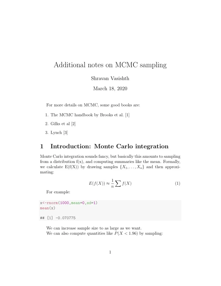
Additional notes on MCMC sampling Shravan Vasishth March 18, 2020 For more details on MCMC, some good books are: 1. The MCMC handbook by Brooks et al. [1] 2. Gilks et al [2] 3. Lynch [3] 1 Introduction: Monte Carlo integration Monte Carlo integration sounds fancy, but basically this amounts to sampling from a distribution f(x), and computing summaries like the mean. Formally, we calculate E(f(X)) by drawing samples { X 1 , . . . , X n } and then approxi- mating: E ( f ( X )) ≈ 1 � f ( X ) (1) n For example: x<-rnorm(1000,mean=0,sd=1) mean(x) ## [1] -0.070775 We can increase sample size to as large as we want. We can also compute quantities like P ( X < 1 . 96) by sampling: 1

mean((x<1.96)) ## [1] 0.977 ## theoretical value: pnorm(1.96) ## [1] 0.975 So, we can compute summary statistics using simulation. However, if we only know up to proportionality the form of the distribution to sample from, how do we get these samples to summarize from? Monte Carlo Markov Chain (MCMC) methods provide that capability: they allow you to sample from distributions you only know up to proportionality. 1.1 Markov chain sampling We have been doing non-Markov chain sampling when we started this course. Taking independent samples is an example of non-Markov chain sampling: indep.samp<-rnorm(500,mean=0,sd=1) head(indep.samp) ## [1] 0.15233 1.46564 2.56170 0.51310 -0.30232 1.01722 The vector of values sampled here are statistically independent. plot(1:500,indep.samp,type="l") 2

3 2 1 indep.samp 0 −1 −2 −3 0 100 200 300 400 500 1:500 If the current value influences the next one, we have a Markov chain. Here is a simple Markov chain: the i-th draw is dependent on the i-1 th draw: nsim<-500 x<-rep(NA,nsim) y<-rep(NA,nsim) x[1]<-rnorm(1) ## initialize x for(i in 2:nsim) { ## draw i-th value based on i-1-th value: y[i]<-rnorm(1,mean=x[i-1],sd=1) x[i]<-y[i] 3

} plot(1:nsim,y,type="l") 20 15 y 10 5 0 0 100 200 300 400 500 1:nsim 1.1.1 What is convergence in a Markov chain? An illustration using discrete Markov chains A discrete Markov chain defines probabilistic movement from one state to the next. Suppose we have 6 states; a transition matrix can define the probabilities: 4

## Set up transition matrix: T<-matrix(rep(0,36),nrow=6) diag(T)<-0.5 offdiags<-c(rep(0.25,4),0.5) for(i in 2:6) { T[i,i-1]<-offdiags[i-1] } offdiags2<-c(0.5,rep(0.25,4)) for(i in 1:5) { T[i,i+1]<-offdiags2[i] } T ## [,1] [,2] [,3] [,4] [,5] [,6] ## [1,] 0.50 0.50 0.00 0.00 0.00 0.00 ## [2,] 0.25 0.50 0.25 0.00 0.00 0.00 ## [3,] 0.00 0.25 0.50 0.25 0.00 0.00 ## [4,] 0.00 0.00 0.25 0.50 0.25 0.00 ## [5,] 0.00 0.00 0.00 0.25 0.50 0.25 ## [6,] 0.00 0.00 0.00 0.00 0.50 0.50 Note that the rows sum to 1, i.e., the probability mass is distributed over all possible transitions from any one location: rowSums(T) ## [1] 1 1 1 1 1 1 We can represent a current location as a probability vector: e.g., in state one, the transition probabilities for possible moves are: T[1,] ## [1] 0.5 0.5 0.0 0.0 0.0 0.0 We can also simulate a random walk based on T: 5

nsim<-500 s<-rep(0,nsim) ## initialize: s[1]<-3 for(i in 2:nsim) { s[i]<-sample(1:6,size=1,prob=T[s[i-1],]) } plot(1:nsim,s,type="l") 6 5 4 s 3 2 1 0 100 200 300 400 500 1:nsim Note that the above random walk is non-deterministic: if we rerun the 6

above code multiple times, we will get different patterns of movement. This Markov chain converges to a particular distribution of probabilities of visiting states 1 to 6. We can see the convergence happen by examining the proportions of visits to each state after blocks of steps that increase by 500 steps: nsim<-50000 s<-rep(0,nsim) ## initialize: s[1]<-3 for(i in 2:nsim) { s[i]<-sample(1:6,size=1,prob=T[s[i-1],]) } blocks<-seq(500,50000,by=500) n<-length(blocks) ## store transition probs over increasing blocks: store.probs<-matrix(rep(rep(0,6),n),ncol=6) ## compute relative frequencies over increasing blocks: for(i in 1:n) { store.probs[i,]<-table(s[1:blocks[i]])/blocks[i] } ## convergence for state 1: for(j in 1:6) { if(j==1) { plot(1:n,store.probs[,j],type="l",lty=j,xlab="block", ylab="probability") } else { lines(1:n,store.probs[,j],type="l",lty=j) } } 7

0.100 0.095 0.090 probability 0.085 0.080 0.075 0 20 40 60 80 100 block Note that each of the rows of the store.probs matrix is a probability mass function, which defines the probability distribution for the 6 states: store.probs[1,] ## [1] 0.098 0.164 0.204 0.200 0.224 0.110 This distribution is settling down to a particular set of values; that’s what we mean by convergence. This particular set of values is: 8

(w<-store.probs[n,]) ## [1] 0.10146 0.19412 0.19228 0.20386 0.20594 0.10234 w is called a stationary distribution. If wT = w , then then w is the stationary distribution of the Markov chain. round(w%*%T,digits=2) ## [,1] [,2] [,3] [,4] [,5] [,6] ## [1,] 0.1 0.2 0.2 0.2 0.21 0.1 round(w,digits=2) ## [1] 0.10 0.19 0.19 0.20 0.21 0.10 This discrete example gives us an intuition for what will happen in con- tinuous distributions: we will devise a Markov chain such that the chain will converge to the distribution we are interested in sampling from. 2 Monte Carlo sampling Suppose we have a posterior that has the form of a Beta distribution. We can sample from the posterior distribution easily: x<-rbeta(5000,1498,1519) Once we have these samples, we can compute any kind of useful summary, e.g., the posterior probability p (given the data) that p > 0 . 5: table(x>0.5)[2]/ sum(table(x>0.5)) ## TRUE ## 0.3394 Or we can compute an interval over which we are 95% sure that the true parameter value lies: 9

##lower bound: quantile(x,0.025) ## 2.5% ## 0.47888 ## upper bound: quantile(x,0.975) ## 97.5% ## 0.51432 Since we can integrate the Beta distribution analytically, we could have done the same thing with the qbeta function (or simply using calculus): (lower<-qbeta(0.025,shape1=1498,shape2=1519)) ## [1] 0.47869 (upper<-qbeta(0.975,shape1=1498,shape2=1519)) ## [1] 0.51436 Using calculus (well, we are still using R; I just mean that one could do this by hand, by solving the integral): integrate(function(x) dbeta(x,shape1=1498,shape2=1519), lower=lower,upper=upper) ## 0.95 with absolute error < 9.9e-12 However—and here we finally get to the crucial point—integration of posterior densities is often impossible (e.g., because they may have many dimensions). In those situations we use sampling methods called Markov chain Monte Carlo, or MCMC, methods. First, let’s look at two relatively simple methods of sampling. 10

3 The inversion method This method works when we can know the closed form of the pdf we want to simulate from and can derive the inverse of that function. Steps: � z 1. Sample one number u from Unif (0 , 1). Let u = F ( z ) = L f ( x ) dx (here, L is the lower bound of the pdf f). 2. Then z = F − 1 ( u ) is a draw from f ( x ). 1 Example: let f ( x ) = 40 (2 x + 3), with 0 < x < 5. We have to draw a number from the uniform distribution and then solve for z, which amounts to finding the inverse function: � z 1 u = 40(2 x + 3) (2) 0 u<-runif(1000,min=0,max=1) z<-(1/2) * (-3 + sqrt(160*u +9)) This method can’t be used if we can’t find the inverse, and it can’t be used with multivariate distributions. 4 The rejection method If F − 1 ( u ) can’t be computed, we sample from f ( x ) as follows: 1. Sample a value z from a distribution g ( z ) from which sampling is easy, and for which mg ( z ) > f ( z ) m a constant (3) mg ( z ) is called an envelope function because it envelops f ( z ). 2. Compute the ratio R = f ( z ) (4) mg ( z ) 11

3. Sample u ∼ Unif (0 , 1). 4. If R > u , then z is treated as a draw from f ( x ). Otherwise return to step 1. 1 For example, consider f(x) to be: f ( x ) = 40 (2 x +3), with 0 < x < 5. The maximum height of f ( x ) is 0 . 325 (why? Try evaluating the function at x=5). So we need an envelope function that exceeds 0 . 325. The uniform density Unif (0 , 5) has maximum height 0.2 (why is that?), so if we multiply it by 2 we have maximum height 0 . 4, which is greater than 0 . 325. In the first step, we sample a number x from a uniform distribution Unif(0,5). This serves to locate a point on the x-axis between 0 and 5 (the domain of x ). The next step involves locating a point in the y direction once the x coordinate is fixed. If we draw a number u from Unif(0,1), then mg ( x ) u = 2 ∗ 0 . 2 u is a number between 0 and 2 ∗ 0 . 2. If this number is less than f(x), that means that the y value falls within f(x), so we accept it, else reject. Checking whether mg ( x ) u is less than f ( x ) is the same as checking whether R = f ( x ) /mg ( z ) > u (5) #R program for rejection method of sampling ## From Lynch book, adapted by SV. count<-0 k<-1 accepted<-rep(NA,1000) rejected<-rep(NA,1000) while(k<1001) { z<-runif(1,min=0,max=5) r<-((1/40)*(2*z+3))/(2*.2) if(r>runif(1,min=0,max=1)) { accepted[k]<-z k<-k+1 } else { rejected[k]<-z } count<-count+1 } 12

hist(accepted,freq=F, main="Example of rejection sampling") fn<-function(x) { (1/40)*(2*x+3) } x<-seq(0,5,by=0.01) lines(x,fn(x)) Example of rejection sampling 0.25 0.20 Density 0.15 0.10 0.05 0.00 0 1 2 3 4 5 accepted 13