Markov chain Monte Carlo Reminder Need to sample large, - PowerPoint PPT Presentation

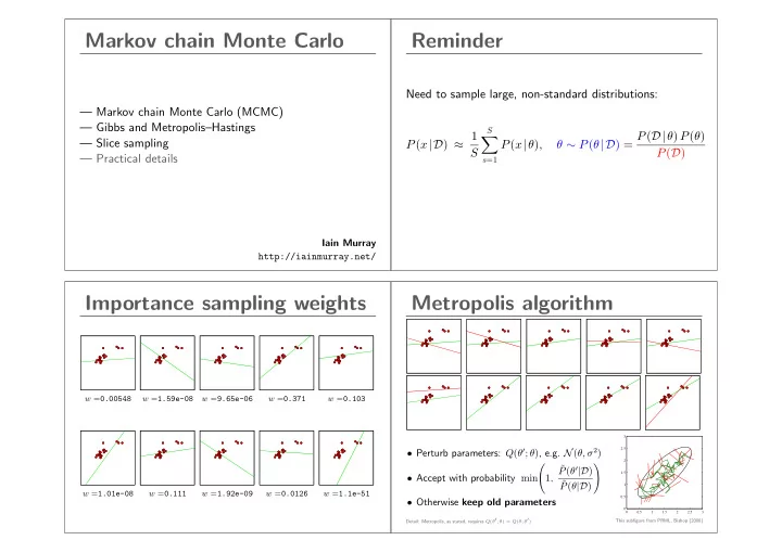
Markov chain Monte Carlo Reminder Need to sample large, non-standard distributions: — Markov chain Monte Carlo (MCMC) — Gibbs and Metropolis–Hastings S θ ∼ P ( θ |D ) = P ( D| θ ) P ( θ ) P ( x |D ) ≈ 1 � — Slice sampling P ( x | θ ) , P ( D ) S — Practical details s =1 Iain Murray http://iainmurray.net/ Importance sampling weights Metropolis algorithm w = 0.00548 w = 1.59e-08 w = 9.65e-06 w = 0.371 w = 0.103 3 2.5 • Perturb parameters: Q ( θ ′ ; θ ) , e.g. N ( θ, σ 2 ) 2 � � ˜ P ( θ ′ |D ) 1.5 • Accept with probability min 1 , ˜ P ( θ |D ) 1 w = 1.01e-08 w = 0.111 w = 1.92e-09 w = 0.0126 w = 1.1e-51 0.5 • Otherwise keep old parameters 0 0 0.5 1 1.5 2 2.5 3 Detail: Metropolis, as stated, requires Q ( θ ′ ; θ ) = Q ( θ ; θ ′ ) This subfigure from PRML, Bishop (2006)

Target distribution Z e − E ( x ) 1 P ( x ) = � e.g. x = E ( x ) = W ij x i x j , x i ∈{± 1 } ( i,j ) ∈ edges > 20,000 citations Local moves Markov chain exploration → → Q ( x ′ ; x ) ւ ↓ ց ↓ Goal: a Markov chain, x t ∼ T ( x t ← x t − 1 ) , such that: P ( x ( t ) ) = e − E ( x ( t ) ) /Z for large t.

Ergodicity Invariant/stationary condition Unique invariant distribution If x ( t − 1) is a sample from P , if ‘forget’ starting point, x (0) x ( t ) is also a sample from P . � T ( x ′ ← x ) P ( x ) = P ( x ′ ) x Gibbs sampling Quick review MCMC: biased random walk exploring a target dist. Pick variables in turn or randomly, and resample P ( x i | x j � = i ) Markov steps, z 2 x ( s ) ∼ T x ( s ) ← x ( s − 1) � � L MCMC gives approximate, correlated samples ? l S E P [ f ] ≈ 1 � f ( x ( s ) ) S s =1 z 1 T must leave target invariant T i ( x ′ ← x ) = P ( x ′ i | x j � = i ) δ ( x ′ j � = i − x j � = i ) T must be able to get everywhere in K steps (for some K )

Gibbs sampling correctness Reverse operators P ( x ) = P ( x i | x \ i ) P ( x \ i ) If T leaves P ( x ) stationary, define a reverse operator T ( x ′ ← x ) P ( x ) x T ( x ′ ← x ) P ( x ) = T ( x ′ ← x ) P ( x ) R ( x ← x ′ ) = . P ( x ′ ) � Simulate by drawing x \ i , then x i | x \ i A necessary condition: there exists R such that: Draw x \ i : sample x , throw initial x i away T ( x ′ ← x ) P ( x ) = R ( x ← x ′ ) P ( x ′ ) , ∀ x, x ′ . If R = T , known as detailed balance (not necessary) Balance condition Metropolis–Hastings 3 2.5 T ( x ′ ← x ) P ( x ) = R ( x ← x ′ ) P ( x ′ ) 2 Arbitrary proposals ∼ Q : 1.5 1 Q ( x ′ ; x ) P ( x ) � = Q ( x ; x ′ ) P ( x ′ ) 0.5 0 0 0.5 1 1.5 2 2.5 3 PRML, Bishop (2006) Satisfies detailed balance by rejecting moves:  � � x ′ � = x 1 , P ( x ′ ) Q ( x ; x ′ ) Q ( x ′ ; x ) min Implies that P ( x ) is left invariant:  P ( x ) Q ( x ′ ; x )  ✯ 1 T ( x ′ ← x ) = ✟ ✟✟✟✟✟✟✟✟✟✟✟✟✟✟✟✟✟ � � T ( x ′ ← x ) P ( x ) = P ( x ′ ) R ( x ← x ′ ) x ′ = x  . . .  x x

Matlab/Octave code for demo Metropolis–Hastings Transition operator function samples = dumb_metropolis(init, log_ptilde, iters, sigma) • Propose a move from the current state Q ( x ′ ; x ) , e.g. N ( x, σ 2 ) D = numel(init); samples = zeros(D, iters); � � 1 , P ( x ′ ) Q ( x ; x ′ ) • Accept with probability min P ( x ) Q ( x ′ ; x ) state = init; • Otherwise next state in chain is a copy of current state Lp_state = log_ptilde(state); for ss = 1:iters Notes % Propose prop = state + sigma*randn(size(state)); • Can use P ∗ ∝ P ( x ) ; normalizer cancels in acceptance ratio Lp_prop = log_ptilde(prop); if log(rand) < (Lp_prop - Lp_state) • Satisfies detailed balance (shown below) % Accept state = prop; • Q must be chosen so chain is ergodic Lp_state = Lp_prop; end � � 1 , P ( x ′ ) Q ( x ; x ′ ) samples(:, ss) = state(:); P ( x ) · T ( x ′ ← x ) = P ( x ) · Q ( x ′ ; x ) min � P ( x ) Q ( x ′ ; x ) , P ( x ′ ) Q ( x ; x ′ ) � = min P ( x ) Q ( x ′ ; x ) end � P ( x ) Q ( x ′ ; x ) � = P ( x ′ ) · Q ( x ; x ′ ) min = P ( x ′ ) · T ( x ← x ′ ) 1 , P ( x ′ ) Q ( x ; x ′ ) Diffusion time Step-size demo Explore N (0 , 1) with different step sizes σ sigma = @(s) plot(dumb_metropolis(0, @(x)-0.5*x*x, 1e3, s)); Generic proposals use P Q ( x ′ ; x ) = N ( x, σ 2 ) sigma(0.1) 4 2 0 99.8% accepts −2 Q σ large → many rejections −4 0 100 200 300 400 500 600 700 800 900 1000 L σ small → slow diffusion: sigma(1) 4 2 ∼ ( L/σ ) 2 iterations required 0 68.4% accepts −2 −4 0 100 200 300 400 500 600 700 800 900 1000 sigma(100) 4 2 0 Adapted from MacKay (2003) 0.5% accepts −2 −4 0 100 200 300 400 500 600 700 800 900 1000

An MCMC strategy Slice sampling idea Sample point uniformly under curve P ∗ ( x ) ∝ P ( x ) Come up with good proposals Q ( x ′ ; x ) ˜ P ( x ) Combine transition operators: ( x, u ) x 1 ∼ T A ( ·← x 0 ) u x 2 ∼ T B ( ·← x 1 ) x x 3 ∼ T C ( ·← x 2 ) p ( u | x ) = Uniform [0 , P ∗ ( x )] x 4 ∼ T A ( ·← x 3 ) x 5 ∼ T B ( ·← x 4 ) � P ∗ ( x ) ≥ u 1 . . . p ( x | u ) ∝ = “Uniform on the slice” 0 otherwise Slice sampling Slice sampling Multimodal conditionals Unimodal conditionals ˜ P ( x ) ( x, u ) ( x, u ) ( x, u ) ( x, u ) u u u x x x u x • bracket slice • place bracket randomly around point • sample uniformly within bracket • shrink bracket if P ∗ ( x ) < u (off slice) • linearly step out until bracket ends are off slice • sample on bracket, shrinking as before • accept first point on the slice Satisfies detailed balance , leaves p ( x | u ) invariant

Slice sampling Summary Advantages of slice-sampling: • We need approximate methods to solve sums/integrals • Easy — only requires P ∗ ( x ) ∝ P ( x ) • Monte Carlo does not explicitly depend on dimension. Using samples from simple Q ( x ) only works in low dimensions. • No rejections • Markov chain Monte Carlo (MCMC) can make local moves. • Tweak params not too important Sample from complex distributions, even in high dimensions. • simple computations ⇒ “easy” to implement (harder to diagnose). There are more advanced versions. Neal (2003) contains many ideas. How should we run MCMC? Forming estimates • The samples aren’t independent. Should we thin , Approximately independent samples can be obtained by thinning . only keep every K th sample? However, all the samples can be used. • Arbitrary initialization means starting iterations are bad. Use the simple Monte Carlo estimator on MCMC samples. It is: Should we discard a “burn-in” period ? — consistent — unbiased if the chain has “burned in” • Maybe we should perform multiple runs? • How do we know if we have run for long enough? The correct motivation to thin: if computing f ( x ( s ) ) is expensive In some special circumstances strategic thinning can help. Steven N. MacEachern and Mario Peruggia, Statistics & Probability Letters, 47(1):91–98, 2000. http://dx.doi.org/10.1016/S0167-7152(99)00142-X — Thanks to Simon Lacoste-Julien for the reference.

Consistency checks Empirical diagnostics Do I get the right answer on tiny versions of my problem? Can I make good inferences about synthetic data drawn from my model? Rasmussen (2000) Recommendations For diagnostics: Getting it right: joint distribution tests of posterior simulators, Standard software packages like R-CODA John Geweke, JASA , 99(467):799–804, 2004. For opinion on thinning, multiple runs, burn in, etc. Practical Markov chain Monte Carlo Posterior Model checking: Gelman et al. Bayesian Data Analysis Charles J. Geyer, Statistical Science . 7(4):473–483, 1992. textbook and papers. http://www.jstor.org/stable/2246094 Summary Getting it right Write down the probability of everything. We write MCMC code to update θ | y θ Condition on what you know, Idea: also write code to sample y | θ sample everything that you don’t. Both codes leave P ( θ, y ) invariant y Samples give plausible explanations: — Look at them Run codes alternately. Check θ ’s match prior — Average their predictions