Bayesian inference & Markov chain Monte Carlo Note 1: Many - PDF document

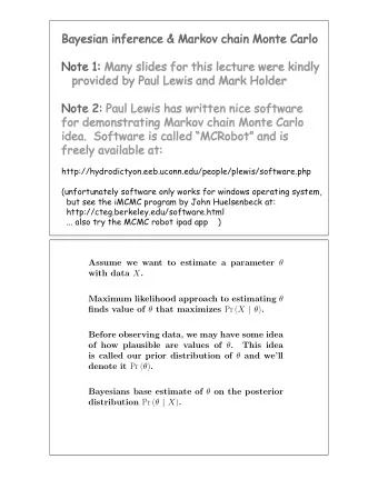
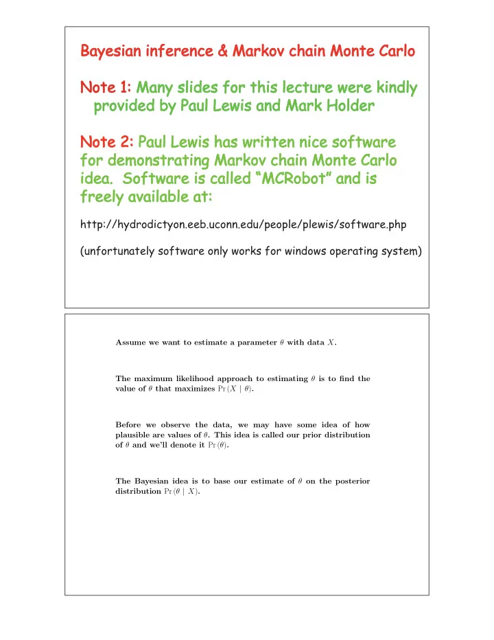
Bayesian inference & Markov chain Monte Carlo Note 1: Many slides for this lecture were kindly provided by Paul Lewis and Mark Holder Note 2: Paul Lewis has written nice software for demonstrating Markov chain Monte Carlo idea. Software is called “MCRobot” and is freely available at: http://hydrodictyon.eeb.uconn.edu/people/plewis/software.php (unfortunately software only works for windows operating system) Assume we want to estimate a parameter θ with data X . The maximum likelihood approach to estimating θ is to find the value of θ that maximizes Pr ( X | θ ) . Before we observe the data, we may have some idea of how plausible are values of θ . This idea is called our prior distribution of θ and we’ll denote it Pr ( θ ) . The Bayesian idea is to base our estimate of θ on the posterior distribution Pr ( θ | X ) .

Pr ( θ | X ) = Pr ( θ, X ) Pr ( X ) = Pr ( X | θ )Pr ( θ ) θ Pr ( X, θ ) dθ � Pr ( X | θ )Pr ( θ ) = θ Pr ( X | θ )Pr ( θ ) dθ � likelihood × prior = difficult quantity to calculate In many situations, determining the exact value of the above integral is difficult. Problems with Bayesian approachs in general: 1. Disagreements about philosophy of inference & Disagreements over priors 2. Heavy Computational Requirements (problem 2 is rapidly becoming less noteworthy)

Potential advantages of Bayesian phylogeny inference Interpretation of posterior probabilities of topologies is more straightforward than interpretation of bootstrap support. If prior distributions for parameters are far from diffuse, very complicated and realistic models can be used and the problem of overparameterization can be simultaneously avoided. MrBayes software for phylogeny inference is at: http://mrbayes.csit.fsu.edu/ Let p be the probability of heads. Then 1-p is the probability of tails Imagine a data set X with these results from flipping a coin Toss 1 2 3 4 5 6 Result H T H T T T Probability p 1-p p 1-p 1-p 1-p 4 2 almost binomial P(X|p) = p (1-p) distribution form

Likelihood with 2 heads and 4 tails 0.020 Likelihood P(X|p) 0.015 0.010 0.005 0.000 0.0 0.2 0.4 0.6 0.8 1.0 p Log-Likelihood with 2 heads and 4 tails Log-Likelihood log(P(X|p)) �5 - �10 - �15 - �20 - �25 - 0.0 0.2 0.4 0.6 0.8 1.0 p

For integers a and b, Beta density B(a,b) is b-1 a-1 P(p)= (a+b-1)!/((a-1)!(b-1)!) p (1-p) where p is between 0 and 1. Expected value of p is a/(a+b) 2 Variance of p is ab/((a+b+1)(a+b) ) � � Beta distribution is conjugate prior for � � � data from binomial distribution Uniform Prior Distribution (i.e., Beta(1,1) distribution) 1.4 1.2 Prior Density P(p) 1.0 0.8 0.6 0.0 0.2 0.4 0.6 0.8 1.0 p

Beta(3,5) posterior from Uniform prior + data (2 heads and 4 tails) 2.0 Posterior P(p|X) 1.5 1.0 0.5 0.0 0.0 0.2 0.4 0.6 0.8 1.0 p Posterior Mean = 3/(3+5) Beta(20,20) prior distribution Prior Mean = 0.5 5 prior density P(p) 4 3 2 1 0 0.0 0.2 0.4 0.6 0.8 1.0 p

Beta(22,24) posterior from Beta(20,20) prior + data (2 heads and 4 tails) 5 Posterior P(p|X) 4 3 2 1 0 0.0 0.2 0.4 0.6 0.8 1.0 p Beta(30,10) prior distribution Prior Mean = 0.75 6 prior density P(p) 5 4 3 2 1 0 0.0 0.2 0.4 0.6 0.8 1.0 p

Beta(32,14) posterior from Beta(30,10) prior + data (2 heads and 4 tails) 6 Posterior Density P(p|X) 5 4 3 2 1 0 0.0 0.2 0.4 0.6 0.8 1.0 p Posterior Mean = 32/(32+14) Likelihood with 20 Heads and 40 Tails Likelihood P(X|p) 2.5e� 17 - 2.0e� 17 - 1.5e� 17 - 1.0e� 17 - 5.0e� 18 - 0.0e+00 0.0 0.2 0.4 0.6 0.8 1.0 p

Log-Likelihood with 20 heads and 40 tails Log-Likelihood log(P(X|p)) �50 - �100 - �150 - �200 - �250 - 0.0 0.2 0.4 0.6 0.8 1.0 p Uniform Prior Distribution (i.e., Beta(1,1) distribution) 1.4 1.2 Prior Density P(p) 1.0 0.8 0.6 0.0 0.2 0.4 0.6 0.8 1.0 p

Beta(21,41) posterior from Uniform prior + data (20 heads and 40 tails) 6 Posterior P(p|X) 5 4 3 2 1 0 0.0 0.2 0.4 0.6 0.8 1.0 p Beta(20,20) prior distribution Prior Mean = 0.5 5 prior density P(p) 4 3 2 1 0 0.0 0.2 0.4 0.6 0.8 1.0 p

Beta(40,60) posterior from Beta(20,20) prior + data (20 heads and 40 tails) 8 Posterior P(p|X) 6 4 2 0 0.0 0.2 0.4 0.6 0.8 1.0 p Beta(30,10) prior distribution Prior Mean = 0.75 6 prior density P(p) 5 4 3 2 1 0 0.0 0.2 0.4 0.6 0.8 1.0 p

Beta(50,50) posterior from Beta(30,10) prior + data (20 heads and 40 tails) 8 Posterior P(p|X) 6 4 2 0 0.0 0.2 0.4 0.6 0.8 1.0 p The Markov chain Monte Carlo (MCMC) idea is to approximate Pr ( θ | X ) by sampling a large number of θ values from Pr ( θ | X ) . So, θ values with a higher posterior probability are more likely to be sampled than θ values with a low posterior probability. Question: How is this sampling achieved? Answer: A Markov chain is constructed and simulated. The states of this chain represent values of θ . The stationary distribution of this chain is Pr ( θ | X ) . In other words, we start the chain at some initial value of θ . After running the chain for a long enough time, the probability of the chain being at some particular state will be approximately equal to the posterior probability of the state.

Let θ ( t ) be the value of θ after t steps of the Markov chain where θ (0) is the initial value. Each step of the Markov chain involves randomly proposing a new value of θ based on the current value of θ . Call the proposed value θ ∗ . We decide with some probability to either accept θ ∗ as our new state or to reject the proposed θ ∗ and remain at our current state. The Hastings (Hastings 1970) algorithm is a way to make this decision and force the stationary distribution of the chain to be Pr ( θ | X ) . According to the Hastings algorithm, what state should we adopt at step t + 1 if θ ( t ) is the current state and θ ∗ is the proposed state? Let J ( θ ∗ | θ ( t ) ) be the “jumping” distribution, i.e. the probability of proposing θ ∗ given that the current state is θ ( t ) . Define r as Pr ( X | θ ∗ )Pr ( θ ∗ ) J ( θ ( t ) | θ ∗ ) r = � � � � X | θ ( t ) θ ( t ) Pr Pr J ( θ ∗ | θ ( t ) ) With probability equal to the minimum of r and 1 , we set θ ( t +1) = θ ∗ . Otherwise, we set θ ( t +1) = θ ( t ) . For the Hastings algorithm to yield the stationary distribution Pr ( θ | X ) , there are a few required conditions. The most important condition is that it must be possible to reach each state from any other in a finite number of steps. Also, the Markov chain can’t be periodic.

MCMC implementation details: The Markov chain should be run as long as possible. We may have T total samples after running our Markov chain. They would be θ (1) , θ (2) , . . . , θ ( T ) . The first B ( 1 ≤ B < T ) of these samples are often discarded (i.e. not used to approximate the posterior). The period before the chain has gotten these B samples that will be discarded is referred to as the “burn–in” period. The reason for discarding these samples is that the early samples typically are largely dependent on the initial state of the Markov chain and often the initial state of the chain is (either intentionally or unintentionally) atypical with respect to the posterior distribution. θ ( B +1) , θ ( B +2) , θ ( T ) The remaining samples . . . , are used to approximate the posterior distribution. For example, the average among the sampled values for a parameter might be a good estimate of its posterior mean. Paul Lewis’ MCMC Robot Demo Target distribution: • Mixture of bivariate normal “hills” • inner contours: 50% of the probability • outer contours: 95% Proposal scheme: • random direction • gamma-distributed step length (mean 45 pixels, s.d. 40 pixels) • reflection at edges

MCMC robot rules Slightly downhill steps Drastic “off the cliff” are usually accepted downhill steps are almost never accepted With these rules, it is easy to see that the robot tends to stay near the tops of hills Uphill steps are always accepted Burn-in First 100 steps Note that first few steps are not at all representative of the distribution. Starting point

Problems with MCMC approaches: 1. They are difficult to implement. Implementation may need to be clever to be computationally tractable and programming bugs are a serious possibility. 2. For the kinds of complicated situations that biologists face, it may be very difficult to know how fast the Markov chain converges to the desired posterior distribution. There are diagnostics for evaluating whether a chain has converged to the posterior distribution but the diagnostics do not provide a guarantee of convergence. A GOOD DIAGNOSTIC : MULTIPLE RUNS !! Just how long is a long run? What would you conclude about the target distri- bution had you stopped the robot at this point? One way to detect this mistake is to perform several independent runs . Results different among runs? Probably none of them were run long enough!