Lecture 9 Dynamic Multi-Threading Cormen et. al., Chapter 27 - PowerPoint PPT Presentation
Lecture 9 Dynamic Multi-Threading Cormen et. al., Chapter 27 Serial vs. Parallel Algorithms Serial algorithms are suitable for running on sequential uniprocessor computers. These sequential computers are not built anymore. We live in the age
Lecture 9 Dynamic Multi-Threading Cormen et. al., Chapter 27
Serial vs. Parallel Algorithms Serial algorithms are suitable for running on sequential uniprocessor computers. These sequential computers are not built anymore. We live in the age of parallel computers, where multiple instructions are executed at the same time. These parallel computers come in different forms: ■ Single multi core chips. A core is a full-fledged processor. Each core can access a single shared memory. ■ Single multi core chips with accelerators. An accelerator is a special co-processor that can execute certain (simple) codes in parallel, e.g. a vector processor that executes the same instruction on an array of values. ■ Distributed memory multi-computers , where each processor’s memory is private, and processors communicate via an interconnection network. We will concentrate on the first class: multi-core shared memory computers. 2
Dynamic Multithreading Programs can specify parallelism through: 1. Nested Parallelism, where a function call is “spawned”, allowing the caller and spawned function to run in parallel. We also call this Task Parallelism. 2. Loop Parallelism, where the iterations of the loop can execute in parallel. These parallel loop iterations and tasks are executed by “virtual processors” or threads . Exactly when a thread executes and on which core it executes is not decided by the programmer, but by the run time system, which coordinates, schedules and manages the parallel computing resources. This lightens the task of writing parallel programs, as we don’t have to worry about data partitioning (shared memory) and task scheduling. 3
Parallel constructs Parallel tasks are created by a spawn and at the end of the task’s execution synchronized with the parent by a sync. Parallel tasks naturally follow the divide-and-conquer paradigm. Parallel loops are created using parallel and new constructs (later). Removing spawn, sync, parallel and new from the program brings back the original sequential code. There is a growing number of dynamic multi threading platforms. E.g., in cs475 we study OpenMP (open multi processing), built on top of C, C++, or Fortran. 4
The basics of dynamic multithreading Fibonacci sequence: F 0 = 0 F 1 = 1 F n = F n-1 + F n-2 n>1 Simple recursive solution: 4 Fib(n) : 3 2 if n<=1 return n 2 else 1 1 0 x = Fib(n-1) y = Fib(n-2) 1 0 return x+y Why do you not want to compute Fibonacci for large n this way? How many nodes in this tree? (order of magnitude) How would you write an efficient Fibonacci?
Run time of Fib(n) T(n) denotes the run time of Fib(n): T(n) = T(n-1) + T(n-2) + ! (1) the two recursive calls and some constant time split and combine extra work Claim: T(n) = ! (F n ) Proof: strong induction. Base: all constants, OK. Step: assume T(m) = ! (F m ) ≤ aF m -b a,b non negative constants, 0 ≤ m < n Then: T(n) ≤ aF n-1 -b + aF n-2 -b + ! (1) = a(F n-1 +F n-2 ) – b – (b- ! (1)) = aF n - b – (b- ! (1)) ≤ aF n - b In fact, we can show that T(n) = ! ( φ n ) φ = (1+Sqrt(5))/2 (CS420) 6
Parallel Fibonacci P-Fib(n): if n<=1 return n else x = spawn P-Fib(n-1) // spawn y = P-Fib(n-2) // call In a sequential call, the caller waits until the called sync returns, whereas in a parallel spawn, the spawner (parent) return x+y may execute at the same time as spawned (child), until the spawner encounters a sync. spawn: the caller (parent) can compute on in parallel with the called (child); it does not have to, but it may (up to the RTS when and where to schedule tasks) sync: the parent must wait for all its spawned children to have completed, before proceeding. The sync is required to avoid summing x+y, before x is computed return: in addition to explicit sync-s, a return statement executes a sync implicitly, so that the parent waits for its children to complete 7
A Multithreaded execution model The multithreaded computation can be viewed as executing a Directed Acyclic Graph G=(V,E), called computation DAG Box: Procedure instance Light: spawned Example: computation DAG for P-Fib(4) Dark: called in parent Circle is a strand: a sequence of non control instructions Black : base case or code up to spawn P-Fib(4) Grey: call in parent White : code after synch Arrows: control: P-Fib(3) P-Fib(2) spawn, call, sequence, return Fat arrows: critical path: the longest path through the computation P-Fib(1) P-Fib(1) P-Fib(0) P-Fib(2) Work: total number of strands Span: number of strands on a critical path Assuming each strand takes one time unit P-Fib(1) P-Fib(0) (total) work equals 17 time units span equals 8 (#critical path strands) 8
A Multithreaded execution model The multithreaded computation can be viewed as executing a Directed Acyclic Graph G=(V,E), called computation DAG, which is embedded in the call tree. Edge (u,v): u executes before v (u,v) indicates a dependency: if a node (strand) has two successors, one of them is spawned if a strand has multiple predecessors, P-Fib(4) they sync before execution continues If there is a path from u to v, they execute in series, otherwise they execute in parallel P-Fib(3) P-Fib(2) Spawn and call edges point downward. Horizontal (continuation) edges indicate that the parent may keep computing while P-Fib(1) P-Fib(1) P-Fib(0) P-Fib(2) spawn executes. Return edges point up. Execution starts in a single initial strand (which one?) and ends in a single final strand P-Fib(1) P-Fib(0) (which one?) 9
Impact of schedule 1: P-F3 2 Processors 2: P-F2 3 Schedule 1 P2 3 5 7 P1 1 2 4 6 8 9 5 4: P-F1 6: P-F1 ----------------------- time 1 2 3 4 5 6 7: P-F0 8 Schedule 2 P2 3 6 P1 1 2 4 5 7 8 9 ------------------------ time 1 2 3 4 5 6 7 9 Unfolded DAG for PF-3 Idle time : number of empty slots (processor not busy) in schedule schedule 1: 3, schedule 2: 5 10
Performance Measures Work: the total time to execute the program sequentially. Assuming 1 time unit per strand, this is the number of nodes (circles) in the DAG. Span: longest time to execute the strands along any path in the tree, i.e., the number of nodes on the critical of the DAG. The run time of the program depends also on schedule and number of processors. Intuitive interpretation of work and span: work models sequential execution time span models fully parallel execution time 11
Performance Measures: time Work: the total time to execute the program sequentially. Assuming 1 time unit per strand, this is the number of nodes in the DAG. Span: longest path length of the DAG. This is the fully parallel execution time (there are always enough processors to execute a task immediately) T 1 : the time to execute the program with 1 processor (T 1 =work) T P : the time to execute the program with P processors As we have seen, different schedules can sometimes take different time, but we always assume greedy scheduling : if there are ( ≥ 1) strands ready and a processor is available, a strand will be executed. (Which strand depends on the scheduler.) Simplifying assumption: We are assuming no time cost for communication between the strands or memory accesses. We call this model of computation ideal. WHY IDEAL? Because we assume no time cost for memory access or communication between the processors executing the strands 12
Work Law and Span Law Work Law: in one step P processors can do at most P units of work: T P ≥ T 1 /P Span Law: T ∞ : the time to execute the program with unlimited #processors (T ∞ = span) is less or equal the time to execute the program with a fixed #processors P T ∞ ≤ T P or T P ≥ T ∞ 13
Performance Measures: parallelism and speedup S P : speedup with P processors: T 1 / T P . (sometimes called ᴨ (pi)): (Average) Parallelism: T 1 / T ∞ ■ average amount of work that can be done per time step With P processors you can only go P times faster than with 1 processor: S P ≤ P linear speedup: S P = fP (0 < f ≤ 1) ideal speedup: f=1 or S P = P (no idle time, all processors busy all the time) When P > ᴨ there will be idle time and thus no ideal speedup. 14
Exercise Fill in T 1 : 1: P-F3 T ∞ : 2: P-F2 3 ᴨ : 5 4: P-F1 6: P-F1 Is there idle time for: P=1 P=2 P=3 ? 7: P-F0 P 3 8 P 2 P 1 Create a schedule for P=3 Time/speedup p=3 9 T 3: S 3: Unfolded DAG for PF-3 Is T 4 < T 3 ? explain 15
Exercise T 1 : 9 1: P-F3 T ∞ : 6 (nodes on critical path: 1,2,5,7,8,9) ᴨ : 9/6 = 1.5 2: P-F2 3 5 Is there idle time for: 4: P-F1 6: P-F1 P=1 P=2 P=3 ? 7: P-F0 P=3: YES P=2: YES 8 P=1: NO (never for P1) Create a schedule for P=3 6 9 3 5 Unfolded DAG for PF-3 1 2 4 7 8 9 T 3: 6 S 3: 9/6=1.5 Is T 4 < T 3 ? NO The fourth processor is unnecessary. Never are there more than 3 parallel strands. 16
Bound on T P We consider greedy schedulers only. If there are at least P strands available in a time step, all processors execute, and we call this a complete step . If there are fewer than P strands available in a time step, some processors will be idle, and we call that an incomplete step . From the work law we know that at best T P =T 1 /P From the span law we know that at best T P = T ∞ 17
Recommend
More recommend
Explore More Topics
Stay informed with curated content and fresh updates.


