Lecture 23 Spatio-temporal Models Colin Rundel 04/17/2017 1 - PowerPoint PPT Presentation
Lecture 23 Spatio-temporal Models Colin Rundel 04/17/2017 1 Spatial Models with AR time dependence 2 Example - Weather station data ## 6 -7.944444 -6.055556 56 6099462 3184587 ## 7 1.2222222 4.944444 10.888889 -9.111111 -6.388889 133
Lecture 23 Spatio-temporal Models Colin Rundel 04/17/2017 1
Spatial Models with AR time dependence 2
Example - Weather station data ## 6 -7.944444 -6.055556 56 6099462 3184587 ## 7 1.2222222 4.944444 10.888889 -9.111111 -6.388889 133 6051946 3225830 8.555556 ## 8 400 6004871 3275456 -12.611111 -9.055556 -1.6111111 2.555556 ## 5 9.666667 176 6123610 3527665 -11.611111 -9.722222 -1.1666667 2.888889 ## 4 9.888889 157 6157302 3484043 -11.111111 -9.444444 -0.3888889 3.944444 2.0555556 5.555556 11.111111 59 6074601 3136288 2.6111111 6.555556 11.388889 ## # ... with 24 more rows, and 19 more variables: y.6 <dbl>, y.7 <dbl>, y.20 <dbl>, y.21 <dbl>, y.22 <dbl>, y.23 <dbl>, y.24 <dbl> ## # y.14 <dbl>, y.15 <dbl>, y.16 <dbl>, y.17 <dbl>, y.18 <dbl>, y.19 <dbl>, ## # y.8 <dbl>, y.9 <dbl>, y.10 <dbl>, y.11 <dbl>, y.12 <dbl>, y.13 <dbl>, ## # 9.000000 -6.555556 -3.500000 360 6005282 3327413 -12.277778 -9.444444 -1.5000000 2.944444 ## 10 9.611111 -9.944444 -8.944444 -0.2777778 3.555556 160 6174891 3455064 ## 9 3.1666667 6.166667 11.500000 ## 3 -6.277778 -4.111111 Based on Andrew Finley and Sudipto Banerjee’s notes from National Ecological Observatory tbl_df () UTMY UTMX elev ## ## # A tibble: 34 × 27 ne_temp select (1:27) %>% y.2 filter (UTMX > 5.5e6, UTMY > 3e6) %>% data (”NETemp.dat”) library (spBayes) starting in January 2000. NETemp.dat - Monthly temperature data (Celsius) recorded across the Northeastern US Network (NEON) Applied Bayesian Regression Workshop, March 7 - 8, 2013 Module 6 y.1 y.3 1 6245390 3262354 <dbl> ## 2 3.7222222 6.777778 12.555556 -6.388889 -3.611111 102 6094162 3195181 ## 1 <dbl> <dbl> y.4 <dbl> <dbl> <dbl> <dbl> <int> ## y.5 3 ne_temp = NETemp.dat %>%
4 2000−01−01 2000−04−01 3400 3200 temp 20 UTMY/1000 3000 10 2000−07−01 2000−10−01 0 −10 3400 3200 3000 5800 5900 6000 6100 6200 5800 5900 6000 6100 6200 UTMX/1000
Dynamic Linear / State Space Models (time) observation equation evolution equation 5 t y t = F ′ θ t p × 1 + v t 1 × p θ t p × 1 = G t p × p θ + ω t p × 1 t − 1 p × 1 v t ∼ N ( 0 , V t ) ω t ∼ N ( 0 , W t )
DLM vs ARMA v t . ... . ARMA / ARIMA are a special case of a dynamic linear model, for example an . 0 0 0 1 0 y t t v t 0 . 2 v t p i 1 i t i 1 1 0 2 . . . 0 1 . 0 0 6 0 0 0 1 . AR ( p ) can be written as F ′ t = ( 1 , 0 , . . . , 0 ) · · · ϕ 1 ϕ 2 ϕ p − 1 ϕ p · · · · · · G t = · · · ω t = ( ω 1 , 0 , . . . 0 ) , ω 1 ∼ N ( 0 , σ 2 )
DLM vs ARMA . 1 0 0 . . . . ARMA / ARIMA are a special case of a dynamic linear model, for example an ... 0 . . . 0 0 0 1 0 p 0 . 0 1 6 0 AR ( p ) can be written as F ′ t = ( 1 , 0 , . . . , 0 ) · · · ϕ 1 ϕ 2 ϕ p − 1 ϕ p · · · · · · G t = · · · ω t = ( ω 1 , 0 , . . . 0 ) , ω 1 ∼ N ( 0 , σ 2 ) v t ∼ N ( 0 , σ 2 y t = θ t + v t , v ) ∑ θ t = ϕ i θ t − i + ω 1 , ω 1 ∼ N ( 0 , σ 2 ω ) i = 1
u 0 s Dynamic spatio-temporal models 2 0 0 0 0 0, Additional assumptions for t 7 2 The observed temperature at time t and location s is given by y t ( s ) where, y t ( s ) = x t ( s ) β t + u t ( s ) + ϵ t ( s ) ind . ϵ t ( s ) ∼ N ( 0 , τ t ) β t = β t − 1 + η t i . i . d . η t ∼ N ( 0 , Σ η ) u t ( s ) = u t − 1 ( s ) + w t ( s ) ∼ N ( ind . t ) ) w t ( s ) 0 , Σ t ( ϕ t , σ
Dynamic spatio-temporal models 2 2 7 The observed temperature at time t and location s is given by y t ( s ) where, y t ( s ) = x t ( s ) β t + u t ( s ) + ϵ t ( s ) ind . ϵ t ( s ) ∼ N ( 0 , τ t ) β t = β t − 1 + η t i . i . d . η t ∼ N ( 0 , Σ η ) u t ( s ) = u t − 1 ( s ) + w t ( s ) ∼ N ( ind . t ) ) w t ( s ) 0 , Σ t ( ϕ t , σ Additional assumptions for t = 0, β 0 ∼ N ( µ 0 , Σ 0 ) u 0 ( s ) = 0
Variograms by time 8 Jan 2000 Apr 2000 semivariance semivariance 4 4 2 2 0 0 0 50 100 150 200 250 300 0 50 100 150 200 250 300 distance distance Jul 2000 Oct 2000 semivariance semivariance 4 4 2 2 0 0 0 50 100 150 200 250 300 0 50 100 150 200 250 300 distance distance
Data and Model Parameters **Data*: ) sigma.eta.IW = list (2, diag (0.001, n_beta)) tau.sq.IG = list ( rep (2, n_t), rep (2, n_t)), sigma.sq.IG = list ( rep (2, n_t), rep (2, n_t)), phi.Unif = list ( rep (3/(0.9 * max_d), n_t), rep (3/(0.05 * max_d), n_t)), beta.0.Norm = list ( rep (0, n_beta), diag (1000, n_beta)), ) sigma.eta = diag (0.01, n_beta) sigma.sq = rep (1, n_t), tau.sq = rep (1, n_t), beta = rep (0, n_t * n_beta), phi = rep (3/(max_d/2), n_t), starting = list ( **Parameters*: y_t = ne_temp %>% select ( starts_with (”y.”)) %>% as.matrix () 9 coords = ne_temp %>% select (UTMX, UTMY) %>% as.matrix () / 1000 max_d = coords %>% dist () %>% max () n_t = ncol (y_t) n_s = nrow (y_t) n_beta = 2 tuning = list (phi = rep (1, n_t)) priors = list (
Fitting with spDynLM from spBayes ## ... ## ## Number of MCMC samples 10000. ## ## Using the exponential spatial correlation model. ## ## Number of covariates 2 (including intercept if specified). ## ## Number of missing observations 0. ## Model fit with 34 observations in 24 time steps. n_samples = 10000 ## ---------------------------------------- ## General model description ## ---------------------------------------- ## file=”dynlm.Rdata”) save (m, ne_temp, models, coords, starting, tuning, priors, n_samples, cov.model = ”exponential”, n.samples = n_samples, n.report = 1000) starting = starting, tuning = tuning, priors = priors, models = lapply ( paste0 (”y.”,1:24, ”~elev”), as.formula) 10 m = spDynLM ( models, data = ne_temp, coords = coords, get.fitted = TRUE,
11 Lapse Rate Posterior Inference - β s (Intercept) elev 20 −0.0050 post_mean param 10 (Intercept) −0.0075 elev 0 −0.0100 −10 0 5 10 15 20 25 0 5 10 15 20 25 month
12 Posterior Inference - θ Eff. Range phi 600 0.08 0.06 400 0.04 200 param 0.02 post_mean Eff. Range phi sigma.sq tau.sq sigma.sq 5 tau.sq 0.75 4 3 0.50 2 1 0.25 0 0 5 10 15 20 25 0 5 10 15 20 25 month
Posterior Inference - Observed vs. Predicted 13 20 10 y_hat 0 −10 −20 −20 −10 0 10 20 y_obs
Prediction n_samples = 5000 file=”dynlm_pred.Rdata”) save (m_pred, pred, models_pred, coords_pred, y_t_pred, n_samples, cov.model = ”exponential”, n.samples = n_samples, n.report = 1000) starting = starting, tuning = tuning, priors = priors, models_pred, data = pred, coords = coords_pred, get.fitted = TRUE, m_pred = spDynLM ( select (-elev) spPredict does not support spDynLM objects. select (1:15) %>% rbind (ne_temp, .) %>% setNames ( names (ne_temp)) %>% as.data.frame () %>% cbind (elev=0, ., matrix (NA, nrow= length (r), ncol=24)) %>% 14 r = raster (xmn=575e4, xmx=630e4, ymn=300e4, ymx=355e4, nrow=20, ncol=20) pred = xyFromCell (r, 1: length (r)) %>% models_pred = lapply ( paste0 (”y.”,1:n_t, ”~1”), as.formula)
15 20 10 post_mean 0 −10 −10 0 10 20 y_obs
16 Jan 2000 Apr 2000 −8 6 −10 4 2 −12 0 −14 −2 −16 −4 Jul 2000 Oct 2000 20 10 18 8 16 6 14 4 12 2 10 0
Spatio-temporal models for continuous time 17
Additive Models In general, spatiotemporal models will have a form like the following, shared information between space and time). these are straight forward to fit and interpret but are quite limiting (no s t w s t dependence between observations in space and time, The simplest possible spatiotemporal model is one were assume there is no Error Spatiotemporal RE Regression error structure 18 y ( s , t ) = µ ( s , t ) mean structure + e ( s , t ) = x ( s , t ) β ( s , t ) + w ( s , t ) + ϵ ( s , t )
Additive Models In general, spatiotemporal models will have a form like the following, shared information between space and time). these are straight forward to fit and interpret but are quite limiting (no dependence between observations in space and time, The simplest possible spatiotemporal model is one were assume there is no Error Spatiotemporal RE 18 Regression error structure y ( s , t ) = µ ( s , t ) mean structure + e ( s , t ) = x ( s , t ) β ( s , t ) + w ( s , t ) + ϵ ( s , t ) w ( s , t ) = α ( t ) + ω ( s )
Spatiotemporal Covariance Lets assume that we want to define our spatiotemporal random effect to be • Even for modest problems this gets very large (past the point of direct computability). matrix 19 a single stationary Gaussian Process (in 3 dimensions ⋆ ), w ( s , t ) ∼ N ( 0 , Σ ( s , t ) ) where our covariance function depends on both ∥ s − s ′ ∥ and | t − t ′ | , cov ( w ( s , t ) , w ( s ′ , t ′ )) = c ( ∥ s − s ′ ∥ , | t − t ′ | ) • Note that the resulting covariance matrix Σ will be of size n s · n t × n s · n t . • If n t = 52 and n s = 100 we have to work with a 5200 × 5200 covariance
Recommend
More recommend
Explore More Topics
Stay informed with curated content and fresh updates.

