Lecture 2: 4/15/17 Lecturer: C. Seshadhri Scribe: Matthew Gray - PDF document

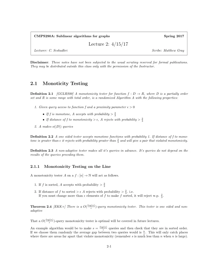
CMPS290A: Sublinear algorithms for graphs Spring 2017 Lecture 2: 4/15/17 Lecturer: C. Seshadhri Scribe: Matthew Gray Disclaimer : These notes have not been subjected to the usual scrutiny reserved for formal publications. They may be distributed outside this class only with the permission of the Instructor. 2.1 Monoticity Testing [GGLRS00] A monotonicity tester for function f : D → R , where D is a partially order Definition 2.1 set and R is some range with total order, is a randomized Algorithm A with the following properties: 1. Given query access to function f and a proximity parameter ǫ > 0 • If f is monotone, A accepts with probability > 2 3 • If distance of f to monotonicity > ǫ , A rejects with probability > 2 3 2. A makes o ( | D | ) queries Definition 2.2 A one sided tester accepts monotone functions with probability 1. If distance of f to mono- tone is greater than ǫ it rejects with probability greater than 2 3 and will give a pair that violated monotonicity. Definition 2.3 A non-adaptive tester makes all it’s queries in advance. It’s queries do not depend on the results of the queries preceding them. 2.1.1 Monotonicity Testing on the Line A monotonicity tester A on a f : [ n ] → N will act as follows. 1. If f is sorted, A accepts with probability > 2 3 2. If distance of f to sorted > ǫ A rejects with probability > 2 3 . i.e. 2 If you must change more than ǫ elements of f to make f sorted, it will reject w.p. 3 . Theorem 2.4 [EKK+] There is a O ( log ( n ) ) -query monotonicity tester. This tester is one sided and non- ǫ adaptive That a O ( log ( n ) )-query monotonicity tester is optimal will be covered in future lectures. ǫ An example algorithm would be to make s = log ( n ) queries and then check that they are in sorted order. ǫ If we choose them randomly the average gap between two queries would is n s . This will only catch places where there are areas far apart that violate monotonicity (remember s is much less than n when n is large). 2-1

2-2 Lecture 2: 4/15/17 If the function is increasing on a large scale but has small dips all over the place a random distribution will not work. So we will instead see if we can try every gap at once. This approach is inspired by Binary Search and has two proofs, one is clean, the other is expressive. We’ll start with the clean one. Here’s the algorithm 1. repeat s ǫ times. (a) Pick x ∈ [ n ] uniform at random (b) Perform Binary Search of f ( x ) on f (c) If you fail to find it successfully REJECT 2. ACCEPT Lemma 2.5 If f is at least ǫ far from monotone, then for at lease ǫn elements in [ n ] , binary search fails. Suppose Lemma is true. If f is monotone, tester always accepts, because a sorted list will never fail a binary search. If the distance from f to monotonicity is > ǫ , then by the Lemma there are > ǫn , where n > 1 elements where binary search fails. Which means that on a single run of the algorithm it fails with probability at least ǫ . So the probability that the tester accepts after s ǫ runs is: Pr [ ACCEPT ] < (1 − ǫ ) s/ǫ lim ǫ → 0 (1 − ǫ ) 1 /ǫ = 1 e Pr [ ACCEPT ] < (1 e ) s = e − s < 1 3 So when ǫ is small and f is at least ǫ far from monotone it fails with probability greater than 2 3 . We still need the lemma so lets prove it. Proof: Lemma 2.5 Suppose that x < y but f ( x ) > f ( y ). Consider the tree generated by a binary search on the domain. x and y have a least common ancestor z. x ≤ z ≤ y but f ( x ) > f ( y ) therefor f ( x ) > f ( z ) or f ( y ) < f ( z ). Which means that binary search will go the wrong way and miss either f ( x ) or f ( y ). Define x to be bad if binary search on x fails. Let B be the set of bad indices. Then f : [ n ] |B , or f on the line without all bad indices, is monotone. [ n ] |B is an increasing subsequence with cardinality | [ n ] |B| ≤ (1 − ǫ ) n when |B| ≥ ǫn . So that was cool and slick, but doesn’t tell you too much about why the tester works. This other proof and algorithm gives you more insight into why monotonicity testers for the line work. Before we get to the algorithm we need some definitions and lemmas. Definition 2.6 The violation graph V G f has vertex cover set [ n ] and an edge ( x, y ) for all pairs x < y, f ( x ) > f ( y ) . Note: this definition works on posets as well as the line. Definition 2.7 ǫ f is the distance of f to monotonicity. Definition 2.8 A Vertex Cover of graph G is a set of vertexes S such that for all edges(u,v) in G { u, v }∪ S � = ∅ .

Lecture 2: 4/15/17 2-3 Lemma 2.9 [FLN+02] The size of the minimum vertex cover of V G f = ǫ f | D | where D is the domain. Proof: Lemma 2.9 Take any vertex cover S of the violation graph V G f . f evaluated on D | S has no violations. It’s possible to “fill in” values in S, so that the resulting function g is monotone. Therefore | S | ≥ ǫ f ∗ D By our previous argument, the number of bad indices (where binary search fails) form a vertex cover of V G f thus the number of bad indices ≥ ǫ f ∗ | D | Here’s the algorithm for the monotonicity tester: 1. Repeat 50( logn ǫ ) times (a) Pick uniform at random x ∈ [ n ] (b) Pick uniform at random k ∈ [1 , logn ] (c) Pick +1 or -1 with probability 1 2 (d) Pick uniform at random y ∈ [ x, x + 2 k ] if 3 was +1 or ∈ [ x − 2 k , x ] if 3 was -1 (e) If (x,y) is a violation REJECT 2. ACCEPT Definition 2.10 x is heavy if there exists x ′ > x such that at least half of the elements of [ x, x ′ ] are in violation with x . Analogously for x ′ < x . Lemma 2.11 Heavy vertices form a vertex cover of V G f Proof: Lemma 2.11 For x < yf ( x ) > f ( y ) then every mid point x < z < y is in violation with either x or y . Thus either x or y is heavy. The powers of 2 give good approximations for the range x ′ that has > 1 2 violations. Let k be the smallest integer k such that 2 k > | x − x ′ | . 2 k is less than 2 | x − x ′ | because 2 k − 1 was less than | x − x ′ | . So | x − x ′ | < 2 k < 2 | x − x ′ | . So if x is heavy the range from x of 2 k in the correct direction will have at least 2 k 1 4 violations. So the probability for finding a violation using the above algorithm is the product of making a good guess at each of the 4 steps. 1. Probability of guessing a heavy x ≥ ǫ 1 2. Probability of guessing a correct k ≥ logn 3. Probability of guessing a correct direction ≥ 1 2 4. Probability of guessing a elem that is in violation ≥ 1 4 ǫ So the probability for finding a violation on one round is ≥ 8 logn Theorem 2.12 The tester works.

2-4 Lecture 2: 4/15/17 Proof: Let us lower bound the probability of rejection if f is ǫ far from monotonic. For each heavy vertex x, there exists some power of 2 such that either [ x − 2 k , x ] or [ x, x + 2 k ] has at least a 1 4 fraction of violations with x. There are at least ǫ heavy x’s because the heavy x’s form a vertex cover of the violation graph. And removing the members of a violation graph would make the function monotonic. ǫ So with the chance of the tester discovering a violation in one round is as shown above to be at least 8 logn , 8 logn ) 50( logn ) which is small. the chance of the algorithm giving a false positive on 50( logn ǫ ǫ ) runs is (1 − ǫ [GGLRS00] O. Goldreich, S. Goldwasser, E. Lehman, D. Ron, and A. Samordinsky , Testing Monotonicity, Combinatorica (2000), pp. 301-337. vol. 20 [FLN+02] E. Fischer E. Lehman I. Newman S. Raskhodnikova R. Rubinfeld , Monotonicity Testing over General Poset Domains, Proceedings of the 34th Annual ACM Symposium on the Theory of Computing (STOC) (2000), pp. 474-483. [EKK+98] Viswanathan , Spot-checkers, Pro- F. ErgnS. Kannan S. KumarR. Rubinfeld M. ceedings of the 30th Annual ACM Symposium on the Theory of Computing (STOC) (1998), pp. 259-268