Lecture 12 Bellman-Ford, Floyd-Warshall, and Dynamic Programming! - PowerPoint PPT Presentation
Lecture 12 Bellman-Ford, Floyd-Warshall, and Dynamic Programming! Announcements HW5 due Friday Midterms have been graded! Pick up your exam after class . Average: 84, Median: 87 Max: 100 (x4) I am very happy with how well
Lecture 12 Bellman-Ford, Floyd-Warshall, and Dynamic Programming!
Announcements • HW5 due Friday • Midterms have been graded! • Pick up your exam after class . • Average: 84, Median: 87 • Max: 100 (x4) • I am very happy with how well y’all did! • Regrade policy: • Write out a regrade request as you would on Gradescope. • Hand your exam and your request to me after class on Wednesday or in my office hours Tuesday (or by appointment).
Last time • Dijkstra’s algorithm! • Solves single-source shortest path in weighted graphs. u s 3 32 1 5 1 b v 13 a 2 2 1 16 t
Today • Bellman-Ford algorithm • Another single-source shortest path algorithm • This is an example of dynamic programming • We’ll see what that means • Floyd-Warshall algorithm • An “all-pairs” shortest path algorithm • Another example of dynamic programming
• Weights on edges Recall represent costs. • The cost of a path is the • A weighted directed graph: sum of the weights along that path. • A shortest path from s u to t is a directed path s 3 32 from s to t with the 1 smallest cost. 5 1 • The single-source This is a b v shortest path problem is 13 path from to find the shortest path s to t of a 21 2 cost 22. from s to v for all v in the graph. 16 t This is a path from s to t of cost 10. It is the shortest path from s to t.
One drawback to Dijkstra • Might not work with negative edge weights • On your homework! u s 3 32 -1 5 -1 b v 13 Why would we ever a have negative weights? 21 -2 Negative costs might • mean benefits. eg, it costs me -$2 • 16 t when I get $2.
Bellman-Ford Algorithm • Slower (but arguably simpler) than Dijkstra’s algorithm. • Works with negative edge weights.
*We won’t actually store all these, but let’s pretend we do for now. Bellman-Ford Algorithm • We keep* an array d (k) of length n for each k = 0, 1, …, n-1. Formally, we will maintain d (k) [b] is the cost of the shortest path the loop invariant: from s to b with at most k edges in it, s u v t For example, this is the shortest • for all b in V. d (0) path from s to t with at most two edges in it. 2 s s u v t But it’s not the shortest path • d (1) u from s to t (with any number of 1 edges). s u v t 5 That’s this one . • d (2) 2 t s u v t v -2 d (3)
*We won’t actually store all these, but let’s pretend we do for now. Bellman-Ford Algorithm • We keep* an array d (k) of length n for each k = 0, 1, …, n-1. Formally, we will maintain d (k) [b] is the cost of the shortest path the loop invariant: from s to b with at most k edges in it, s u v t for all b in V. d (0) 0 ∞ ∞ ∞ 0 s 2 s u v t ∞ d (1) u 1 s u v t 5 d (2) 2 t s u v t v -2 d (3) ∞ ∞
While maintaining: Now update! d (k) [b] is the cost of the shortest path from s to b with at most k edges in it. • We will use the table d (0) to fill in d (1) • Then use d (1) to fill in d (2) • … • Then use d (k-1) to fill in d (k) • ... • Then use d (n-2) to fill in d (n-1) This eventually gives us what we want: • d (k) [a] is the shortest path from s to a with at most k edges. • Eventually we’ll get all the shortest paths…
How do we get d (k) [b] from d (k-1) ? Want to maintain: d (k) [b] is the cost of the shortest path • Two cases: from s to b with at most k edges in it. Case 1 : the shortest path from s to b with at most k edges actually has at most k-1 edges. d (k) [b] = d (k-1) [b] 2 b s 2 u say k=3 Case 2 : the shortest path from s to b with at most k edges really has k edges. d (k) [b] = d (k-1) [a] + w(a,b) for some a... 2 a 2 d (k) [b] = min a {d (k-1) [a] + w(a,b)} x 2 10 b s 2 u say k=3
Bellman-Ford Algorithm* • Bellman-Ford*(G,s): • Initialize d (k) for k = 0, …, n-1 • d (0) [v] = ∞ for all v other than s This minimum is over • d (0) [s] = 0. all a so that (a,b) is in E • For k = 1, …, n-1: • For b in V: • d (k) [b] ← min{ d (k-1) [b], min a {d (k-1) [a] + weight(a,b)} } • Return d (n-1) If we set d (k) [b] to be the minimum of the previous two cases, then we maintain the loop invariant that: d (k) [b] is the cost of the shortest path from s to b with at most k edges in it.
Bellman-Ford Algorithm* Example d (k) [b] is the cost of the shortest path from s to b with at most k edges in it. • For k = 1,…,n-1: • For b in V: • d (k) [b] ← min{ d (k-1) [b], min a {d (k-1) [a] + weight(a,b)} } s u v t d (0) 0 ∞ ∞ ∞ 0 s 2 s u v t ∞ d (1) u 1 s u v t 5 d (2) 2 t s u v t v -2 d (3) ∞ ∞
Bellman-Ford Algorithm* Example d (k) [b] is the cost of the shortest path from s to b with at most k edges in it. • For k = 1,…,n-1: • For b in V: • d (k) [b] ← min{ d (k-1) [b], min a {d (k-1) [a] + weight(a,b)} } s u v t d (0) 0 ∞ ∞ ∞ 0 s 2 s u v t 2 d (1) 0 2 5 ∞ u 1 s u v t 5 d (2) 2 t s u v t v -2 d (3) ∞ 5
Bellman-Ford Algorithm* Example d (k) [b] is the cost of the shortest path from s to b with at most k edges in it. • For k = 1,…,n-1: • For b in V: • d (k) [b] ← min{ d (k-1) [b], min a {d (k-1) [a] + weight(a,b)} } s u v t d (0) 0 ∞ ∞ ∞ 0 s 2 s u v t 2 d (1) 0 2 5 ∞ u 1 s u v t 5 d (2) 0 2 4 3 2 t s u v t v -2 d (3) 3 4
Bellman-Ford Algorithm* Example d (k) [b] is the cost of the shortest path from s to b with at most k edges in it. • For k = 1,…,n-1: • For b in V: • d (k) [b] ← min{ d (k-1) [b], min a {d (k-1) [a] + weight(a,b)} } s u v t d (0) 0 ∞ ∞ ∞ 0 s 2 s u v t 2 d (1) 0 2 5 ∞ u 1 s u v t 5 d (2) 0 2 4 3 2 t s u v t v -2 d (3) 2 4 0 2 4 2
Bellman-Ford Algorithm* Example d (k) [b] is the cost of the shortest path from s to b with at most k edges in it. SANITY CHECK: • The shortest path with 1 edge from s to t has cost ∞. (there is no such path). • The shortest path with 2 edges from s to t has cost 3. (s-v-t) • The shortest path with 3 edges from s to t has cost 2. (s-u-v-t) And this one is the shortest path!!! s u v t d (0) 0 ∞ ∞ ∞ 0 s 2 s u v t 2 d (1) 0 2 5 ∞ u 1 s u v t 5 d (2) 0 2 4 3 2 t s u v t v -2 d (3) 2 4 0 2 4 2
How do we actually implement this? (This is what the * on all the previous slides was for). • Don’t actually keep all the arrays d (k) around. • Just keep two of them at a time, that’s all we need. • Running time: O(mn) • That’s worse than Dijkstra, but BF can handle negative edge weights. • Space complexity: • We need space to store the graph and two arrays of size n. *WARNING: This is slightly different from the version of Bellman-Ford in CLRS. But we will stick with what we just saw for pedagogical reasons. See Lecture Notes 11.5 (listed on the webpage in the Lecture 12 box) for notes on the analysis of the slightly different CLRS version.
Bellman-Ford Algorithm* • Bellman-Ford*(G,s): • Initialize d (k) for k = 0, …, n-1 • d (0) [v] = ∞ for all v other than s • d (0) [s] = 0. • For k = 1, …, n-1: • For b in V: • d (k) [b] ← min{ d (k-1) [b], min a {d (k-1) [a] + weight(a,b)} } • Return d (n-1)
Why does it work? • First, we’ve been asserting that: d (n-1) [b] is the cost of the shortest path from s to b with at most n-1 edges in it. • Technically, this requires proof! • We’ve basically already seen the proof! • It follows from induction with the inductive hypothesis d (k) [b] is the cost of the shortest path Work out the details of this proof from s to b with at most k edges in it. on your own! To help you, there’s an outline on the next slide. (Which we’ll skip now).
Sketch of proof [skip this in lecture] that this thing we’ve been asserting is really true • Inductive hypothesis: d (k) [b] is the cost of the shortest path from s to b with at most k edges in it. • Base case: For k = 0: 0 ∞ ∞ ∞ Case 2 : the shortest path from s to b of length at most k edges has • Inductive step: exactly k edges • d (k) [b] ← min{ d (k-1) [b], min a {d (k-1) [a] + weight(a,b)} } Case 1 : the shortest path from s to be has <k edges • In either case, we make the correct update. When k = n-1, the inductive hypothesis reads: • Conclusion: d (n-1) [b] is the cost of the shortest path from s to b with at most n-1 edges in it.
Is this the conclusion we want? d (n-1) [b] is the cost of the shortest path from s to b with at most n-1 edges in it. • We still need to prove that this implies BF* is correct. • We return d (n-1) • Need to show d (n-1) [a] = distance(s,a). • Enough to show: Shortest path with at Shortest path with any most n-1 edges number of edges
Recommend
More recommend
Explore More Topics
Stay informed with curated content and fresh updates.


