Lecture 10: Linear Discriminant Functions (contd.) Perceptron Aykut - PowerPoint PPT Presentation
Lecture 10: Linear Discriminant Functions (contd.) Perceptron Aykut Erdem November 2016 Hacettepe University Last time Logistic Regression Assumes%the%following%func$onal%form%for%P(Y|X):% Assumes the following functional form for
Lecture 10: − Linear Discriminant Functions (cont’d.) − Perceptron Aykut Erdem November 2016 Hacettepe University
Last time… Logistic Regression Assumes%the%following%func$onal%form%for%P(Y|X):% Assumes the following functional form for P(Y|X): Logis$c%func$on%applied%to%a%linear% Logistic function applied to linear func$on%of%the%data% function of the data logit%(z)% Logis&c( Logistic func&on( function slide by Aarti Singh & Barnabás Póczos (or(Sigmoid):( (or Sigmoid): z% Features(can(be(discrete(or(con&nuous!( Features can be discrete or continuous! 8% 2
Last time.. LR vs. GNB • LR is a linear classifier − decision rule is a hyperplane • LR optimized by maximizing conditional likelihood − no closed-form solution − concave ! global optimum with gradient ascent • Gaussian Naïve Bayes with class-independent variances representationally equivalent to LR − Solution di ff ers because of objective (loss) function • In general, NB and LR make di ff erent assumptions − NB: Features independent given class! assumption on P( X |Y) slide by Aarti Singh & Barnabás Póczos − LR: Functional form of P(Y| X ), no assumption on P( X |Y) • Convergence rates − GNB (usually) needs less data − LR (usually) gets to better solutions in the limit 3
Last time… Linear Discriminant Function • Linear discriminant function for a vector x y ( x ) = w T x + w 0 where w is called weight vector, and w 0 is a bias. • The classification function is C ( x ) = sign ( w T x + w 0 ) where step function sign(·) is defined as ( + 1 , a > 0 sign ( a ) = − 1 , a < 0 slide by Ce Liu 4
Last time… Properties of Linear Discriminant Functions • The decision surface, shown in red, x 2 y > 0 is perpendicular to w , and its y = 0 R 1 displacement from the origin is y < 0 R 2 controlled by the bias paramete r w 0 . • The signed orthogonal distance of x a general point x from the decision w y ( x ) surface is given by y ( x )/|| w || k w k x ? • y ( x ) gives a signed measure of the perpendicular distance r of the x 1 point x from the decision surface � w 0 k w k • y( x ) = 0 for x on the decision surface. The normal distance from the origin to the decision surface is w T x k w k = � w 0 k w k slide by Ce Liu • So w 0 determines the location of the decision surface. the decision surface. 5
Last time… Multiple Classes: Simple Extension • One-versus-the-rest classifier: classify C k and samples not in C k . • One-versus-one classifier: classify every pair of classes. C 3 C 1 ? R 1 R 3 R 1 C 1 ? R 2 C 3 C 1 R 2 R 3 C 2 C 2 not C 1 slide by Ce Liu C 2 not C 2 6
Last time… Multiple Classes: K-Class Discriminant • A single K -class discriminant comprising K linear functions y k ( x ) = w T k x + w k 0 • Decision function C ( x ) = k , if y k ( x ) > y j ( x ) 8 j 6 = k • The decision boundary between class C k and C j is given by y k ( x ) = y j ( x ) C C ( w k � w j ) T x + ( w k 0 � w j 0 ) = 0 slide by Ce Liu 7
Today • Properties of Linear Discriminant Functions (cont’d.) • Perceptron 8
Property of the Decision Regions Theorem The decision regions of the K-class discriminant y k ( x ) = w T k x + w k 0 are singly connected and convex. Proof. Suppose two points x A and x B both lie inside decision region R k . Any point ˆ x on the line between x A and x B can be expressed as ˆ x = λ x A + ( 1 � λ ) x B So y k (ˆ x ) = λ y k ( x A ) + ( 1 � λ ) y k ( x B ) > λ y j ( x A ) + ( 1 � λ ) y j ( x B ) ( 8 j 6 = k ) = y j (ˆ x ) ( 8 j 6 = k ) Therefore, the regions R k is single connected and convex. slide by Ce Liu 9
Property of the Decision Regions Theorem The decision regions of the K-class discriminant y k ( x ) = w T k x + w k 0 are singly connected and convex. Proof. Suppose two points x A and x B both lie inside decision region R k . Any point ˆ x on the line between x A and x B can be expressed as ˆ x = λ x A + ( 1 � λ ) x B So y k (ˆ x ) = λ y k ( x A ) + ( 1 � λ ) y k ( x B ) > λ y j ( x A ) + ( 1 � λ ) y j ( x B ) ( 8 j 6 = k ) = y j (ˆ x ) ( 8 j 6 = k ) Therefore, the regions R k is single connected and convex. slide by Ce Liu 10
Property of the Decision Regions Theorem The decision regions of the K-class discriminant y k ( x ) = w T k x + w k 0 are singly connected and convex. If two points x A and x B both lie ul- inside the same decision region decision R k , then any point x that lies on R j the line connecting these two re- points must also lie in R k , and line R i hence the decision region must in be singly connected and be convex. R k x B x A ˆ x slide by Ce Liu 11
Fisher’s Linear Discriminant • Pursue the optimal linear projection on which the two classes can be maximally separated A way to view a linear y = w T x classification model is in • The mean vectors of the two classes terms of dimensionality reduction. m 1 = 1 m 2 = 1 X X x n , x n N 1 N 2 n ∈ C 1 n ∈ C 2 4 4 2 2 0 0 − 2 − 2 slide by Ce Liu − 2 2 6 − 2 2 6 Di ff erence of means Fisher’s Linear Discriminant 12
What’s a Good Projection? • After projection, the two classes are separated as much as possible. Measured by the distance between projected center ⌘ 2 ⇣ w T ( m 1 − m 2 ) = w T ( m 1 − m 2 )( m 1 − m 2 ) T w = w T S B w where S B = ( m 1 − m 2 )( m 1 − m 2 ) T is called between-class covariance matrix. • After projection, the variances of the two classes are as small as possible. Measured by the within-class covariance where w T S W w ( x n − m 1 )( x n − m 1 ) T + X X ( x n − m 2 )( x n − m 2 ) T S W = slide by Ce Liu n ∈ C 1 n ∈ C 2 13
Fisher’s Linear Discriminant Fisher criterion: maximize the ratio w.r.t. w • Within-class variance = w T S B w J ( w ) = Between-class variance w T S W w for f ( x ) = g ( x ) Recall the quotient rule: for • h ( x ) f 0 ( x ) = g 0 ( x ) h ( x ) � g ( x ) h 0 ( x ) h 2 ( x ) Setting ∇ J ( w ) = 0 , we obtain • ( w T S B w ) S W w = ( w T S W w ) S B w ⇣ ⌘ ( w T S B w ) S W w = ( w T S W w )( m 2 � m 1 ) ( m 2 � m 1 ) T w Terms w T S B w , w T S W w and ( m 2 − m 1 ) T w are scalars, and we only care • about directions. So the scalars are dropped. Therefore slide by Ce Liu w / S � 1 W ( m 2 � m 1 ) 14
From Fisher’s Linear Discriminant to Classifiers • Fisher’s Linear Discriminant is not a classifier; it only decides on an optimal projection to convert high-dimensional classification problem to 1D. • A bias (threshold) is needed to form a linear classifier (multiple thresholds lead to nonlinear classifiers). The final classifier has the form y ( x ) = sign ( w T x + w 0 ) where the nonlinear activation function sign(·) is a step · function ( + 1 , a > 0 sign ( a ) = − 1 , a < 0 • How to decide the bias w 0 ? slide by Ce Liu 15
Perceptron 16
early theories of the brain slide by Alex Smola
Biology and Learning • Basic Idea - Good behavior should be rewarded, bad behavior punished (or not rewarded). This improves system fitness. - Killing a sabertooth tiger should be rewarded ... - Correlated events should be combined. - Pavlov’s salivating dog. • Training mechanisms - Behavioral modification of individuals (learning) Successful behavior is rewarded (e.g. food). - Hard-coded behavior in the genes (instinct) The wrongly coded animal does not reproduce. slide by Alex Smola 18
Neurons • Soma (CPU) Cell body - combines signals • Dendrite (input bus) Combines the inputs from several other nerve cells • Synapse (interface) Interface and parameter store between neurons • Axon (cable) May be up to 1m long and will transport the activation slide by Alex Smola signal to neurons at di ff erent locations 19
Neurons x n x 1 x 2 x 3 . . . w n w 1 synaptic weights output X slide by Alex Smola f ( x ) = w i x i = h w, x i i 20
Perceptron • Weighted linear x 3 x n x 1 x 2 . . . combination w n w 1 • Nonlinear synaptic decision function weights • Linear o ff set (bias) output f ( x ) = σ ( h w, x i + b ) • Linear separating hyperplanes (spam/ham, novel/typical, click/no click) • Learning slide by Alex Smola Estimating the parameters w and b 21
Perceptron Ham Spam slide by Alex Smola 22
Perceptron Widom Rosenblatt slide by Alex Smola
The Perceptron initialize w = 0 and b = 0 repeat if y i [ h w, x i i + b ] 0 then w w + y i x i and b b + y i end if until all classified correctly • Nothing happens if classified correctly X • Weight vector is linear combination w = y i x i • Classifier is linear combination of i ∈ I inner products X f ( x ) = y i h x i , x i + b slide by Alex Smola i ∈ I 24
Convergence Theorem • If there exists some with unit length and ( w ∗ , b ∗ ) y i [ h x i , w ∗ i + b ∗ ] � ρ for all i then the perceptron converges to a linear separator after a number of steps bounded by b ∗ 2 + 1 ⇣ ⌘ � r 2 + 1 ρ − 2 where k x i k r � • Dimensionality independent • Order independent (i.e. also worst case) • Scales with ‘di ffi culty’ of problem slide by Alex Smola 25
Recommend
More recommend
Explore More Topics
Stay informed with curated content and fresh updates.

