Lecture 10 : Continuous Random Variables 0/ 21 In this section you - PowerPoint PPT Presentation
Lecture 10 : Continuous Random Variables 0/ 21 In this section you will compute probabilities by doing integrals. Definition A random variable X is said to be continuous if there exists a nonnegative function f ( x ) definition interval (
Lecture 10 : Continuous Random Variables 0/ 21
In this section you will compute probabilities by doing integrals. Definition A random variable X is said to be continuous if there exists a nonnegative function f ( x ) definition interval ( −∞ , ∞ ) such that for any interval [ a , b ] we have, b � P ( a ≤ X ≤ b ) = f ( x ) dx a 1/ 21 Lecture 10 : Continuous Random Variables
Definition (Cont.) f ( x ) is said to be the probability density function of X, abbreviated pdf. � b a f ( x ) dx as the area between The usual geometric interpretation of the integral a and b under the graph of f will be very important later h p a r g o f 2/ 21 Lecture 10 : Continuous Random Variables
Z f ( x ) � P ( X = x ) in fact f ( x ) is not the probability of anything f is a density i.e., something you integrate to get the magnitude of a physical quantity. Think of a wire stretching from a to b with density λ gm cm � b a λ ( x ) dx . Then the actually mass of the wire between a and b is 3/ 21 Lecture 10 : Continuous Random Variables
So λ is mass per unit length λ ( x ) = lim △ m △ x Similarly f ( x ) = probability per unit length. So both λ ( x ) resp. f ( x ) are densities which must be integrated to get the actual length resp. probability. Properties of f ( x ) (i) f ( x ) ≥ 0 ← no immediate physic interpretation, see later. � ∞ (ii) −∞ f ( x ) dx = 1 ← total probability = 1 Any function f ( x ) satisfying (i) and (ii) is a probability density function. 4/ 21 Lecture 10 : Continuous Random Variables
Example : The Uniform Distribution on [ 0 , 1 ] Physical Problem Pick a random number in [ 0 , 1 ] Call the result X . So X is a random variable. Questions � � X = 1 What is P ? 2 � � 0 ≤ X ≤ 1 What is P 2 � 1 � 4 ≤ X ≤ 3 What is P 4 5/ 21 Lecture 10 : Continuous Random Variables
So for any interval [ a , b ] which is a subinterval of [ 0 , 1 ] we have the formula � b P ( X ∈ [ a , b ]) = P ( a ≤ X ≤ b ) = 1 dx = b − a = length ([ a , b ]) a This is a continuous random variable. The density function is the “characteristic function of [ 0 , 1 ] ” i.e., � 1 , 0 ≤ x ≤ 1 f ( x ) = 0 , otherwise. 0 1 6/ 21 Lecture 10 : Continuous Random Variables
Definition A continuous random variable X is said to have uniform distribution on [ 0 , 1 ] , abbreviate X ∼ U ( 0 , 1 ) if its pdf f is given by 1 , 0 ≤ x ≤ 1 f ( x ) = 0 , otherwise. More generally suppose we replace [ 0 , 1 ] by the interval [ a , b ] Z We can’t have 1 , a ≤ x ≤ b ✘ f ( x ) = ✘✘✘✘✘✘✘✘ 0 , otherwise. 7/ 21 Lecture 10 : Continuous Random Variables
Why? 1 So we have to define 1 � a ≤ x ≤ b b − a , f ( x ) = 0 , otherwise � b a f ( x ) dx = 1 Then 8/ 21 Lecture 10 : Continuous Random Variables
Another Example Linear density 0 1 Consider the function � 2 x , 0 ≤ x ≤ 1 f ( x ) = 0 , otherwise Then the total probability is x = 1 � 1 ∞ � � � � 2 x = ( x 2 ) � f ( x ) dx = = 1 � � � � −∞ 0 � x = 0 9/ 21 Lecture 10 : Continuous Random Variables
Since f ( x ) ≥ 0 and ∞ � f ( x ) dx = 1 −∞ f ( x ) is indeed a pdf. Problem For the linear density compute � 1 � 4 ≤ X ≤ 3 P 4 Solution 3 ∞ 4 � 1 � � � 4 ≤ X ≤ 3 P = f ( x ) dx = 2 xdx 4 −∞ 1 4 x = 3 = 9 16 − 1 16 = 1 � = ( x 2 ) 4 � � 2 � x = 1 4 No decimals please. 10/ 21 Lecture 10 : Continuous Random Variables
Here are some usual properties of continuous random variables. They are all consequences of the fact that if X is continuous and c is any number then P ( X = c ) = 0 So if X is a continuous random variable, all point probabilities are zero. Theorem (i) P ( a ≤ X ≤ b ) = P ( a ≤ X < b ) (because P ( X = b ) = 0 ) (ii) P ( a ≤ X ≤ b ) = P ( a < X ≤ b ) (because P ( X = a ) = 0 ) (iii) P ( a ≤ X ≤ b ) = P ( a < X < b ) end points don’t matter. 11/ 21 Lecture 10 : Continuous Random Variables
Good Citizen Computations The Cumulative Distribution Function Definition Let X be a continuous random variable with pdf f. Then the cumulative distribution function F, abbreviate cdf, is defined by x � F ( x ) = f ( x ) dx −∞ = the area under the graph of f to the left of x. 12/ 21 Lecture 10 : Continuous Random Variables
This area is We will compute the cdfs for X ∼ U ( 0 , 1 ) and X ∼ the linear distribution. X ∼ U ( 0 , 1 ) 1 0 1 13/ 21 Lecture 10 : Continuous Random Variables
There will be three formulas corresponding to the two discontinuities in f ( x ) . F ( x ) = 0, x < 0 This is clear because we haven’t accumulated any probability/area get. no area 1 F ( x ) = 1, x > 1 This is not quite so clean area 1 to the left 1 1 1 We have area 1 to the left of x and that’s all we are going to get no matter how far we push the vertical line to the right. 14/ 21 Lecture 10 : Continuous Random Variables
F ( x ) =? , 0 ≤ x ≤ 1 This is where the action is. 1 How much area have we accumulated to the left of x . It is the area of a rectangle with base x and height 1 hence area x · 1 = x . Thus F ( x ) = x , 0 ≤ x ≤ 1 We could have done this with integrals instead of pictures but pictures are better. 15/ 21 Lecture 10 : Continuous Random Variables
We have obtained 0 , x < 0 F ( x ) = x , 0 ≤ x ≤ 1 1 , x > 1 1 Lesson cdf ’s of continuous random variables are continuous and satisfy x →−∞ F ( x ) = 0 lim x →∞ F ( x ) = 1 lim 16/ 21 Lecture 10 : Continuous Random Variables
The cdf of the linear distribution 1 We will go faster. Clearly again F ( x ) = 0 , x < 0 F ( x ) = 1 , and x > 1 We have to compute F ( x ) for 0 ≤ x ≤ 1. 17/ 21 Lecture 10 : Continuous Random Variables
So we have to compute the area of a triangle with base b = x and height h = 2 x . But = 1 2 bh = 1 2 x ( 2 x ) = x 2 area So 0 , x < 0 x 2 , F ( x ) = 0 ≤ x ≤ 1 1 , x > 1 Do this with integrals. 18/ 21 Lecture 10 : Continuous Random Variables
Importance of the cdf Coded into the cdf F are all the probabilities P ( a ≤ X ≤ b ) . Theorem P ( a ≤ X ≤ b ) = F ( b ) − F ( c ) . Proof. P ( a ≤ X ≤ b ) = P ( X ≤ b ) − P ( X < a ) But because X is continuous P ( X < a ) = P ( X ≤ a ) So P ( a ≤ X ≤ b ) = P ( X ≤ b ) − P ( X ≤ 0 ) = F ( b ) − F ( a ) � 19/ 21 Lecture 10 : Continuous Random Variables
Remark The previous theorem is critical. It is the basis of using tables (in a book or in a computer) to compute probabilities. A grid of values of F (up to 10 decimal places say) are tabulated. Theorem (How to recover the pdf from the cdf ) F ′ ( x ) = f ( x ) at all points where f ( x ) is continuous. 20/ 21 Lecture 10 : Continuous Random Variables
Example Suppose X ∼ U ( 0 , 1 ) hence F ( x ) has the graph 0 1 So F ( x ) is differentiable except at 0 and 1 and has derivative 1 But this is f ( x ) . Note f ( x ) is discontinuous of 0 and 1 . 21/ 21 Lecture 10 : Continuous Random Variables
Recommend
More recommend
Explore More Topics
Stay informed with curated content and fresh updates.
