Probability and Statistics for Computer Science Can we call - PowerPoint PPT Presentation
Probability and Statistics for Computer Science Can we call the e exci-ng ? e n 1 + 1 e = lim n n Credit: wikipedia Hongye Liu, Teaching Assistant Prof, CS361, UIUC, 10.1.2020 Thurs Oct . 8 Midterm 1 . . (
Probability and Statistics ì for Computer Science Can we call the e exci-ng ? e � n � 1 + 1 e = lim n n →∞ Credit: wikipedia Hongye Liu, Teaching Assistant Prof, CS361, UIUC, 10.1.2020
Thurs Oct . 8 Midterm 1 . . ( CBT F ) 12 : 30pm & alternative conflicts CBTF 8 Oct 8pm → , 9 , CBTF 8 am Oct → . 4pm 8 , Oct instructions , practices check out .
Last time Poisson Distribution Variable Random continuous Function probability Density
Objectives Distribution Function Cumulative variable random continuous for C Gaussian ) Distribution Normal Pdt P ' " ' Distribution Exponential y f poxidx =/ - o
Function Distribution Cumulative P ( X E x ) Det . : PCXEXK.IE?pcX=x ) Discrete Rv . - S -2 RV continuous → ¥1,1 pcxex ) =) × pix , dx " ^ - x
Cumulative distribution of continuous uniform distribution � Cumula-ve distribu-on func-on (CDF) � x P ( X ≤ x ) = p ( x ) dx −∞ of a uniform random variable X is: CD Ffx=¥ ] CDF = o . 5 p ( x ) 1 -m¥ 1 I b − a 1 too --T x_ a 0 a 0 a b X b X ,
Q: Probability density function: spinner � What is the constant c given the spin angle θ - has the following pdf? is the CDF ? what , p ( θ ) A. 1 a B. 1/π C. 2/π ÷ c D. 4/π , E. 1/2π π 0 2π θ
Quantile µ Pdf Cx ) ( DF l K ) - 7 o ( K Go . 7 4. on to 7
Normal (Gaussian) distribution � The most famous con-nuous random variable distribu-on. The probability density is this: [ Trix ) dx 2 π exp ( − ( x − µ ) 2 1 p ( x ) = ) √ - b = / 2 σ 2 or σ - ( exp ) → e # - E 2 e Carl F. Gauss ¥ (1777-1855) Credit: wikipedia
Normal (Gaussian) distribution � The most famous con-nuous random variable distribu-on. The probability density is this: 2 π exp ( − ( x − µ ) 2 1 p ( x ) = ) √ 2 σ 2 σ E [ X ] = µ & var [ X ] = σ 2 Carl F. Gauss (1777-1855) Credit: wikipedia
Normal (Gaussian) distribution � A lot of data in nature are approximately normally distributed, ie. Adult height , etc. 2 π exp ( − ( x − µ ) 2 1 p ( x ) = ) √ 2 σ 2 σ E [ X ] = µ & var [ X ] = σ 2 Carl F. Gauss (1777-1855) Credit: wikipedia
PDF and CDF of normal distribution curves probability density tune . I ( PDF ) ← | § " " " " " " " € Cumin FIT fun . . g- + ( CDF ) E " T ; into µ =o I • • 0=1 I I ' all Credit: wikipedia @
Quantile) CK , → Pdf � Quan(les)give) Probability)density) a)measure)of) - loca(on,)the) / median)is)the) , 0.5)quan(le) → CDF ✓ 2=0.253 OFI Cumula(ve)Probability) ) )(CDF))) fo . 6=0.253 - ← y ÷ Credit:)) J.)Orloff)et)al) )))
Q.) � What)is)the)value)of)50%)quan(le)in)a) - standard)normal)distribu(on?) A. J1) B. 0) " C. 1)
Spread of normal (Gaussian) distributed data 99.7% 95% 68% res f p CX ) DX e. 68 µ - 6 6 si : .mx I . . . . Credit: wikipedia
Standard normal distribution � If we standardize the normal distribu-on (by subtrac-ng μ and dividing by σ), we get a random variable that has standard normal x - U distribu-on. = si g- � A con-nuous random variable X is standard normal if 2 π exp ( − x 2 1 p ( x ) = 2 ) √ -
Derivation of standard normal distribution - ⇐ Ki . � + ∞ Sakae x = x − µ ˆ p ( x ) dx σ −∞ � + ∞ e- ¥ 2 π exp ( − ( x − µ ) 2 1 = ) dx ¥ dx = √ 2 σ 2 σ , −∞ � + ∞ x 2 1 2 π exp ( − ˆ = 2 ) σ d ˆ x √ σ Call this standard and omit −∞ � + ∞ x 2 2 π exp ( − ˆ 1 using a hat = 2 ) d ˆ x √ −∞ � + ∞ 2 π exp ( − x 2 1 = p (ˆ x ) dx p ( x ) = 2 ) −∞ √
C D F C b ) - CDF Ca ) ¥*¥÷t¥ peaks D= fab -¥ . doc
I rat a . . stuff cos . zico # It cPFy;¥tfma ②
Q. What is the mean of standard normal? e A. 0 B. 1
Q. What is the standard deviation of standard normal? A. 0 B. 1 a
Standard normal distribution � If we standardize the normal distribu-on (by subtrac-ng μ and dividing by σ), we get a random variable that has standard normal distribu-on. � A con-nuous random variable X is standard normal if 2 π exp ( − x 2 1 p ( x ) = 2 ) √ E [ X ] = 0 & var [ X ] = 1
Another way to check the spread of normal distributed data � Frac-on of normal data within 1 standard 1=5 devia-on from the mean. � 1 exp ( − x 2 1 2 ) dx ≃ 0 . 68 √ 2 π − 1 � Frac-on of normal data within k standard devia-ons from the mean. � k exp ( − x 2 1 2 ) dx √ 2 π − k
Using the standard normal’s table to calculate for a normal distribution’s probability � If X ~ N (μ=3, σ 2 =16) (normal distribu-on) ✓ O - 5 → I ss P ( X ≤ 5) =? # . ÷÷÷ If - - -
Q. � If X ~ N (μ=3, σ 2 =16) (normal distribu-on) a- A . 0.5199 B. 0.5987 C. 0.6915 P ( X ≤ 5) =?
Q. Is the table with only positive x values enough? e A. Yes B. No.
Central limit theorem (CLT) � The distribu-on of the sum of N independent iden-cal (IID) random variables tends toward a normal distribu-on as N ∞ � Even when the component random variables are not exactly IID, the result is approximately OI = CDF a S true and very useful in prac-ce " # - t XN S = X i t Xu - - s → - µ → s , tinsel S n I → E c Norma ,
Central limit theorem (CLT) � CLT helps explain the prevalence of normal distribu-ons in nature � A binomial random variable tends toward a normal distribu-on when N is large due to the fact it is the sum of IID Bernoulli random variables
The Binomial distributed beads of the Galton Board The Binomial distribu-on looks very similar to Normal when N is large
Binomial approximation with Normal ' * minor " - k Htt pix-ks-cyeypkci.pt e- pea > = Fo Binomial distribu-on Approxima-on with Normal i Y Bernoulli Binomial Normal XB = 0.20 0.20 n=20,p=0.5 n=20,p=0.7 ● μ = 20, σ 2 = 10 n=40,p=0.5 ● ● GI var ● ● ● 0.15 0.15 n= 40, p=0.5 ÷÷÷÷÷÷¥÷÷÷.¥¥h pix ● ● ● ● ● ● ● ● ● ● probability probability 0.10 0.10 ● ● ● ● ● ● ● ● ● ● ● ● ● ● ● ● 0.05 0.05 ● ● ● ● ● ● ● ● ● ● ● ● ● ● ● ● ● ● ● ● 0.00 ● ● ● ● ● ● ● ● ● ● ● ● ● ● ● ● ● ● ● ● ● ● ● ● ● ● ● ● 0.00 ● ● ● ● ● ● ● ● ● ● ● ● ● ● ● ● ● ● ● ● ● ● ● ● ● ● ● ● ● ● ● ● ● ● ● ● ● ● ● ● ● ● ● ● ● ● ● ● ● ● ● ● ● ● ● ● ● ● ● ● ● ● ● ● ● ● ● ● ● ● ● ● ● ● ● ● ● ● ● ● ● ● ● ● 0 10 20 30 40 0 10 20 30 40 k k
Binomial approximation with Normal � Let k be the number of heads appeared in 40 tosses of fair coin � The goal is to es-mate the following with normal 25 � 40 � � 0 . 5 k 0 . 5 40 − k P (10 ≤ k ≤ 25) = k k =10 25 � 40 � 0 . 5 40 ≃ 0 . 96 � = k k =10 � E [ k ] = np = 40 · 0 . 5 = 20 std [ k ] = np (1 − p ) - - √ √ = 40 · 0 . 5 · 0 . 5 = 10
Binomial approximation with Normal � Use the same mean and standard devia-on of the original binomial distribu-on. √ JV ( o , I ) µ = 20 σ = 10 ≃ 3 . 16 . � Then standardize the normal to do the calcula-on PEEL � 25 exp ( − ( x − µ ) 2 1 P (10 ≤ k ≤ 25) ≃ ) dx √ 2 σ 2 2 π σ 10 25 − 20 exp ( − x 2 1 � 3 . 16 = 2 ) dx √ ii. 2 π 10 − 20 3 . 16 ≃ 0 . 94
Exponential distribution � Common p ( x ) = λ e − λ x for x ≥ 0 Model for wai-ng -me � Associated with the Poisson distribu-on with the same λ Credit: wikipedia
Exponential distribution � A con-nuous random variable X is exponen-al if it represent the “-me” un-l next incident in a Poisson distribu-on with intensity λ . Proof See Degroot et al Pg 324. p ( x ) = λ e − λ x for x ≥ 0 � It’s similar to Geometric distribu>on – the discrete version of wai-ng in queue
Expectations of Exponential distribution � A con-nuous random variable X is exponen-al if it represent the “-me” un-l next incident in a Poisson distribu-on with intensity λ . p ( x ) = λ e − λ x for x ≥ 0 E [ X ] = 1 & var [ X ] = 1 x λ 2 λ
Example of exponential distribution � How long will it take un-l the next call to be received by a call center? Suppose it’s a random variable T . If the number of incoming call is a Poisson distribu-on with intensity λ = 20 in an hour . What is the expected -me for T?
Q: � A store has a number of customers coming on Sat. that can be modeled as a Poisson distribu-on. In order to measure the average rate of customers in the day, the staff recorded the -me between the arrival of customers, can he reach the same goal? A. Yes B. No
Additional References � Charles M. Grinstead and J. Laurie Snell "Introduc-on to Probability” � Morris H. Degroot and Mark J. Schervish "Probability and Sta-s-cs”
See you next time See You!
Recommend
More recommend
Explore More Topics
Stay informed with curated content and fresh updates.
