General structure Here we suppose that the consequences are wealth - PDF document

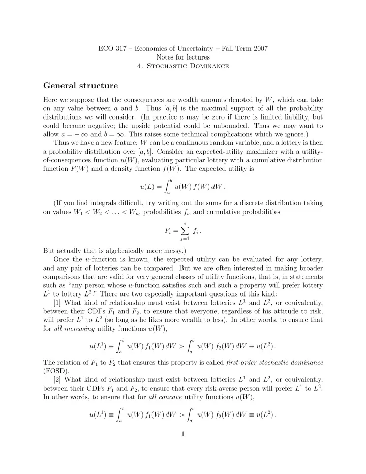
ECO 317 – Economics of Uncertainty – Fall Term 2007 Notes for lectures 4. Stochastic Dominance General structure Here we suppose that the consequences are wealth amounts denoted by W , which can take on any value between a and b . Thus [ a, b ] is the maximal support of all the probability distributions we will consider. (In practice a may be zero if there is limited liability, but could become negative; the upside potential could be unbounded. Thus we may want to allow a = − ∞ and b = ∞ . This raises some technical complications which we ignore.) Thus we have a new feature: W can be a continuous random variable, and a lottery is then a probability distribution over [ a, b ]. Consider an expected-utility maximizer with a utility- of-consequences function u ( W ), evaluating particular lottery with a cumulative distribution function F ( W ) and a density function f ( W ). The expected utility is � b u ( L ) = a u ( W ) f ( W ) dW . (If you find integrals difficult, try writing out the sums for a discrete distribution taking on values W 1 < W 2 < . . . < W n , probabilities f i , and cumulative probabilities i � F i = f i . j =1 But actually that is algebraically more messy.) Once the u -function is known, the expected utility can be evaluated for any lottery, and any pair of lotteries can be compared. But we are often interested in making broader comparisons that are valid for very general classes of utility functions, that is, in statements such as “any person whose u -function satisfies such and such a property will prefer lottery L 1 to lottery L 2 .” There are two especially important questions of this kind: [1] What kind of relationship must exist between lotteries L 1 and L 2 , or equivalently, between their CDFs F 1 and F 2 , to ensure that everyone, regardless of his attitude to risk, will prefer L 1 to L 2 (so long as he likes more wealth to less). In other words, to ensure that for all increasing utility functions u ( W ), � b � b u ( L 1 ) ≡ a u ( W ) f 2 ( W ) dW ≡ u ( L 2 ) . a u ( W ) f 1 ( W ) dW > The relation of F 1 to F 2 that ensures this property is called first-order stochastic dominance (FOSD). [2] What kind of relationship must exist between lotteries L 1 and L 2 , or equivalently, between their CDFs F 1 and F 2 , to ensure that every risk-averse person will prefer L 1 to L 2 . In other words, to ensure that for all concave utility functions u ( W ), � b � b u ( L 1 ) ≡ a u ( W ) f 2 ( W ) dW ≡ u ( L 2 ) . a u ( W ) f 1 ( W ) dW > 1

The relation of F 1 to F 2 that ensures this property is called second-order stochastic dominance (SOSD). Comments: (1) For arbitrary L 1 and L 2 , neither may dominate the other in either of these senses. In other words, both of these dominance concepts are partial orderings of lotteries, not complete orderings. (2) Your first thought may be that first-order stochastic dominance should correspond to having a higher mean, and second-order stochastic dominance should correspond to having a lower variance, but neither of these intuitions is correct. You should be able to see after a moment’s thought that a higher mean is not going to suffice for FOSD: F 1 may have a higher mean but so much higher variance than F 2 that someone with an increasing but concave utility function will like L 1 less than L 2 . But the point about variance and SOSD is more subtle. We will see counterexamples soon. First-Order Stochastic Dominance To find the mathematical concept of FOSD, begin by observing that for any distribution function F and its density function f , and for any utility function u � b � b [ u ( W ) F ( W ) ] b a u ′ ( W ) F ( W ) dW a u ( W ) f ( W ) dW = a − integrating by parts � b a u ′ ( W ) F ( W ) dW = u ( b ) ∗ 1 − u ( a ) ∗ 0 − � b a u ′ ( W ) F ( W ) dW = u ( b ) − Therefore comparing expected utility under two different distributions (if they have different “supports” [ a, b ], take the biggest and define the other density outside its support to be 0): � b � b � b � b a u ( W ) f 1 ( W ) dW − a u ( W ) f 2 ( W ) dW = − a u ′ ( W ) F 1 ( W ) dW + a u ′ ( W ) F 2 ( W ) dW � b = a u ′ ( W ) [ F 2 ( W ) − F 1 ( W ) ] dW . We want this to be positive for all increasing functions u , that is, for all functions with u ′ ( W ) > 0 for all W ∈ [ a, b ]. That will obviously be true if F 2 ( W ) > F 1 ( W ) for all W ∈ ( a, b ). We cannot avoid equality at the endpoints a and b because F 1 ( a ) = F 2 ( a ) = 0 and F 1 ( b ) = F 2 ( b ) = 1. But that does not hurt the result. We can also allow equalities at isolated points within the interval. Again I leave more rigorous proofs to more advanced (graduate) courses. But the converse is also true: if F 2 ( W ) < F 1 ( W ) for any ranges of W ∈ ( a, b ), then we will be able to construct a function u for which u ′ ( W ) is very positive and significant, say equal to 1, in these ranges, and still positive but very small, say some ǫ , everywhere else. By choosing ǫ small enough, we can then make the integral on the right hand side negative. This counterexample shows that F 1 ( W ) < F 2 ( W ) for all W ∈ ( a, b ) is also necessary for u ( L 1 ) > u ( L 2 ) to be true for all increasing u functions. 2

So we have the desired result if, and only if, F 2 ( W ) > F 1 ( W ) for all W ∈ ( a, b ). We might make this our definition of FOSD, and state the result proved in the above argument as a theorem: Definition 1: The distribution F 1 is first-order stochastic dominant over F 2 if and only if F 1 ( W ) < F 2 ( W ) for all W ∈ ( a, b ). Theorem 1: Every expected-utility maximizer with an increasing utility function of wealth prefers the lottery L 1 with distribution F 1 to L 2 with distribution F 2 if and only if F 1 is FOSD over F 2 . Figure 1 shows two such cumulative distribution functions. I have taken a = 0 and b = 1 for convenience. Since both distributions start out at 0 when W = a = 0, and then F 1 ( W ) becomes less than F 2 ( W ), it must be the case that F 1 ( W ) is flatter than F 2 ( W ) for small W . Since the slope of the cumulative distribution function is the probability density function, the density f 1 ( W ) must be less than the density f 2 ( W ) for small W . Conversely, both distributions climb to 1 at W = b = 1, but F 1 ( W ) climbs from smaller values than F 2 ( W ), it must be the case that F 1 ( W ) is steeper than F 2 ( W ) for W close to 1. That is, the density f 1 ( W ) is higher than the density f 2 ( W ) for W close to 1. Figure 2 shows the density functions. F(x) 1 F (x) 2 F (x) 1 x 1 Figure 1: FOSD: CDF comparison f(x) 2 f (x) f (x) 2 1 1 x 1 Figure 2: FOSD: Density comparison The density comparison can be restated as saying: f 1 ( W ) can be obtained from f 2 ( W ) 3

by shifting some probability weight from lower to higher values of W . That is an intuition for why anyone who prefers more wealth to less prefers the lottery L 1 to L 2 . For your information, the functions are f 1 ( W ) = 12 W 2 (1 − W ) , f 2 ( W ) = 12 W (1 − W ) 2 , F 1 ( W ) = 4 W 3 − 3 W 4 , F 2 ( W ) = 6 W 2 − 8 W 3 + 3 W 4 . Second-Order Stochastic Dominance The procedure is similar except that we have to integrate by parts twice. Write � W S ( W ) = F ( w ) dw . a This is the integral of the cumulative distribution function, so its value at any point W is the area under the F ( w ) curve for w going from a to W . And by the fundamental theorem of the calculus, the cumulative distribution function is its derivative: F ( W ) = S ′ ( W ) for all W . Call the S function the “super-cumulative” distribution function for short. Note that S ( a ) = 0. Now carry out the process of integration by parts twice: � b � b [ u ( W ) F ( W ) ] b a u ( W ) f ( W ) dW = a − a u ′ ( W ) F ( W ) dW integrating by parts � b = u ( b ) ∗ 1 − u ( a ) ∗ 0 − a u ′ ( W ) F ( W ) dW � b = u ( b ) − a u ′ ( W ) F ( W ) dW � b u ( b ) − [ u ′ ( W ) S ( W ) ] b = a + a u ′′ ( W ) S ( W ) dW int. by parts again � b = u ( b ) − u ′ ( b ) S ( b ) + a u ′′ ( W ) S ( W ) dW Therefore � b � b a u ( W ) f 1 ( W ) dW − a u ( W ) f 2 ( W ) dW � b u ′ ( b ) [ S 2 ( b ) − S 1 ( b )] + a u ′′ ( W ) [ S 1 ( W ) − S 2 ( W )] dW = We want our dominance definition to be such that every risk-averse person prefers L 1 and every risk-loving person prefers L 2 . Therefore we want the expression on the right hand side of the last line to be positive for all concave functions u , that is, for all functions with u ′′ ( W ) < 0 for all W ∈ [ a, b ]; we also want the same expression to be negative for all convex functions, that is, for all functions with u ′′ ( W ) > 0. And therefore, on the borderline, we want a risk-neutral person to be indifferent between L 1 and L 2 . That is, the whole expression on the right hand side of the last line should be 4