3.13.3 Binomial Distribution and Discrete Random Variables Prof. - PowerPoint PPT Presentation
3.13.3 Binomial Distribution and Discrete Random Variables Prof. Tesler Math 186 Winter 2017 Prof. Tesler 3.13.3 Binomial Distribution Math 186 / Winter 2017 1 / 16 Random variables A random variable X is a function assigning a real
3.1–3.3 Binomial Distribution and Discrete Random Variables Prof. Tesler Math 186 Winter 2017 Prof. Tesler 3.1–3.3 Binomial Distribution Math 186 / Winter 2017 1 / 16
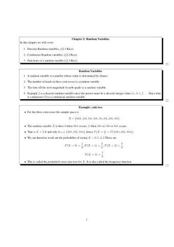
Random variables A random variable X is a function assigning a real number to each outcome in a sample space. A biased coin has probability p of heads, q = 1 − p of tails. Flip the coin 3 times and let X denote the number of heads: X ( HHH ) = 3 X ( HHT ) = X ( HTH ) = X ( THH ) = 2 X ( TTT ) = 0 X ( HTT ) = X ( THT ) = X ( TTH ) = 1 The range of X is { 0 , 1 , 2 , 3 } . The discrete probability density function (pdf) is p X ( k ) = P ( X = k ) : p X ( 0 ) = q 3 p X ( 1 ) = 3 pq 2 p X ( 2 ) = 3 p 2 q p X ( 3 ) = p 3 p X ( k ) is defined for all real numbers k . In this case, p X ( k ) = 0 for k � 0 , 1 , 2 , 3 : p X ( 4 ) = 0 p X ( 2 . 5 ) = 0 p X (− 3 ) = 0 p X ( π ) = 0 . . . Prof. Tesler 3.1–3.3 Binomial Distribution Math 186 / Winter 2017 2 / 16
Discrete random variables In the preceding example, the range of X is a discrete set , not a continuum (such as the real number interval [ 0 , 3 ] ). So X is a discrete random variable . Sometimes it’s called a probability mass function (pmf) in the discrete case, vs. a probability density function (pdf) in the continuous case. We’ll use probability density function for both. Notation p X ( k ) = P ( X = k ) : Use capital letters ( X ) for random variables and lowercase ( k ) to stand for numeric values. A discrete probability density function requires p X ( k ) � 0 for all k , and that the total probability is � k p X ( k ) = 1 . On the previous slide: � p X ( k ) = p X ( 0 ) + p X ( 1 ) + p X ( 2 ) + p X ( 3 ) k = q 3 + 3 pq 2 + 3 p 2 q + p 3 = ( q + p ) 3 = 1 3 = 1 Prof. Tesler 3.1–3.3 Binomial Distribution Math 186 / Winter 2017 3 / 16
Binomial distribution A biased coin has probability p of heads, q = 1 − p of tails. Flip the coin 7 times. P ( HHTHTTH ) = ppqpqqp = p 4 q 3 = p # heads q # tails � 7 � p 4 q 3 P ( 4 heads in 7 flips ) = 4 Flip the coin n times ( n = 0 , 1 , 2 , 3 , . . .). Let X be the number of heads. The probability density function (pdf) of X is � � n � p k q n − k if k = 0 , 1 , . . . , n ; k p X ( k ) = P ( X = k ) = otherwise. 0 Interpretation: Repeat this experiment (flipping a coin n times and counting the heads) a huge number of times. The fraction of experiments with X = k will be approximately p X ( k ) . Prof. Tesler 3.1–3.3 Binomial Distribution Math 186 / Winter 2017 4 / 16
Binomial distribution � � n � p k q n − k if k = 0 , 1 , . . . , n ; k p X ( k ) = P ( X = k ) = otherwise. 0 The range of X is { 0 , 1 , 2 , . . . , n } . p X ( k ) � 0 for all values k . The sum of all probability densities is 1: n � n � � p k q n − k = ( p + q ) n = 1 n = 1 k k = 0 The relationship to the binomial formula is why it’s named the binomial distribution . Prof. Tesler 3.1–3.3 Binomial Distribution Math 186 / Winter 2017 5 / 16
Genetics example Consider pea plants from a Tt × Tt cross. The offspring have Genotype Probability Phenotype 1/4 tall TT 1/2 tall Tt 1/4 short tt so the phenotypes have P ( tall ) = 3 / 4 , P ( short ) = 1 / 4 . If there are 10 offspring, the number X of tall offspring has a binomial distribution with n = 10 , p = 3 / 4 : � � 10 � ( 3 / 4 ) k ( 1 / 4 ) 10 − k if k = 0 , 1 , . . . , 10 ; k p X ( k ) = P ( X = k ) = otherwise. 0 Later: We will see other bioinformatics applications that use the binomial distribution, including genome assembly and Haldane’s model of recombination. Prof. Tesler 3.1–3.3 Binomial Distribution Math 186 / Winter 2017 6 / 16
Binomial distribution for n = 10 , p = 3 / 4 Discrete probability density function pdf k 1 0 0.00000095 0.8 1 0.00002861 2 0.00038624 3 0.00308990 0.6 p X (k) 4 0.01622200 5 0.05839920 0.4 6 0.14599800 7 0.25028229 0.2 8 0.28156757 9 0.18771172 10 0.05631351 0 other 0 0 5 10 k Prof. Tesler 3.1–3.3 Binomial Distribution Math 186 / Winter 2017 7 / 16
Cumulative Distribution Function (cdf) The Cumulative Distribution Function (cdf) of random variable X is F X ( k ) = P ( X � k ) defined over all real numbers k . In our example, F X ( 1 )= P ( X � 1 ) = p X ( 0 ) + p X ( 1 ) = 0 . 00000095 + 0 . 00002861 = 0 . 00002956 F X ( 2 )= P ( X � 2 ) = p X ( 0 ) + p X ( 1 ) + p X ( 2 ) = 0 . 00000095 + 0 . 00002861 + 0 . 00038624 = 0 . 00041580 Alternately: = F X ( 1 ) + p X ( 2 ) = . 00002956 + 0 . 00038624 = 0 . 00041580 Prof. Tesler 3.1–3.3 Binomial Distribution Math 186 / Winter 2017 8 / 16
CDF in-between points with nonzero probability Note that F X ( 1 . 5 ) = P ( X � 1 . 5 ) = p X ( 0 ) + p X ( 1 ) = F X ( 1 ) The binomial distribution has nonzero probability only at integers. In-between integers, PDF: p X ( k ) = 0 CDF: F X ( k ) = F X ( ⌊ k ⌋ ) , where ⌊ k ⌋ is the floor of k (largest integer � k ): ⌊ 3 ⌋ = 3 , ⌊ − 3 ⌋ = − 3 , ⌊ 3 . 2 ⌋ = 3 , ⌊ − 3 . 2 ⌋ = − 4 . Warning Be careful, this is just our first example. If the range of a random variable includes non-integer locations, go down to the largest value � k with nonzero probability instead of to ⌊ k ⌋ . Prof. Tesler 3.1–3.3 Binomial Distribution Math 186 / Winter 2017 9 / 16
CDF outside of the range In this example, the range of X is { 0 , 1 , . . . , 10 } . F X (− 3 . 2 ) = P ( X � − 3 . 2 ) = 0 since minimum X in range is 0. F X ( 12 . 8 ) = P ( X � 12 . 8 ) = 1 since the whole range is � 12 . 8 . This example has a bounded range. F X ( k ) = 0 below the range and F X ( k ) = 1 above the range. But not all random variables have a bounded range. Instead, for any random variable, we have asymptotic results: k → − ∞ F X ( k ) = 0 k → + ∞ F X ( k ) = 1 lim lim As k goes from − ∞ to ∞ , the cdf weakly increases. For a discrete random variable, the cdf jumps where the pdf is nonzero. Prof. Tesler 3.1–3.3 Binomial Distribution Math 186 / Winter 2017 10 / 16
Binomial distribution for n = 10 , p = 3 / 4 pdf p X ( k ) cdf F X ( k ) k k < 0 0 0 0.00000095 0.00000095 0 � k < 1 1 0.00002861 1 � k < 2 0.00002956 2 0.00038624 2 � k < 3 0.00041580 3 0.00308990 0.00350571 3 � k < 4 4 0.01622200 4 � k < 5 0.01972771 5 0.05839920 0.07812691 5 � k < 6 6 0.14599800 6 � k < 7 0.22412491 7 0.25028229 0.47440720 7 � k < 8 8 0.28156757 8 � k < 9 0.75597477 9 0.18771172 9 � k < 10 0.94368649 10 0.05631351 1.00000000 10 � k other 0 Discrete probability density function Cumulative distribution function 1 1 0.8 0.8 0.6 0.6 p X (k) F X (k) 0.4 0.4 0.2 0.2 0 0 0 5 10 0 5 10 k k Prof. Tesler 3.1–3.3 Binomial Distribution Math 186 / Winter 2017 11 / 16
Using pdf and cdf table (binomial n = 10 , p = 3 / 4 ) Different inequality symbols � , > , < , � pdf p X ( k ) cdf F X ( k ) k 0 k < 0 0 0.00000095 0 � k < 1 0.00000095 1 0.00002861 1 � k < 2 0.00002956 2 0.00038624 0.00041580 2 � k < 3 3 0.00308990 3 � k < 4 0.00350571 4 0.01622200 0.01972771 4 � k < 5 5 0.05839920 5 � k < 6 0.07812691 6 0.14599800 6 � k < 7 0.22412491 7 0.25028229 0.47440720 7 � k < 8 8 0.28156757 8 � k < 9 0.75597477 9 0.18771172 0.94368649 9 � k < 10 10 0.05631351 1.00000000 10 � k other 0 P ( X � 2 ) = 0 . 00041580 P ( X > 2 ) = 1 − P ( X � 2 ) = 1 − 0 . 00041580 = 0 . 99958420 P ( X < 2 ) = P ( X � 2 − ) = F X ( 2 − ) = 0 . 00002956 using infinitesimal notation from Calculus: 2 − is just below 2 . P ( X � 2 ) = 1 − P ( X < 2 ) = 1 − F X ( 2 − ) = 0 . 99997044 Prof. Tesler 3.1–3.3 Binomial Distribution Math 186 / Winter 2017 12 / 16
Using pdf and cdf table (binomial n = 10 , p = 3 / 4 ) Probability of an interval pdf p X ( k ) cdf F X ( k ) k 0 k < 0 0 0.00000095 0.00000095 0 � k < 1 1 0.00002861 1 � k < 2 0.00002956 2 0.00038624 0.00041580 2 � k < 3 3 0.00308990 3 � k < 4 0.00350571 4 0.01622200 0.01972771 4 � k < 5 5 0.05839920 5 � k < 6 0.07812691 6 0.14599800 6 � k < 7 0.22412491 7 0.25028229 0.47440720 7 � k < 8 8 0.28156757 8 � k < 9 0.75597477 9 0.18771172 0.94368649 9 � k < 10 10 0.05631351 1.00000000 10 � k other 0 F X ( 4 ) = P ( X � 4 ) = p X ( 0 ) + p X ( 1 ) + p X ( 2 ) + p X ( 3 ) + p X ( 4 ) F X ( 2 ) = P ( X � 2 ) = p X ( 0 ) + p X ( 1 ) + p X ( 2 ) P ( 2 < X � 4 ) = p X ( 3 ) + p X ( 4 ) = P ( X � 4 ) − P ( X � 2 ) = F X ( 4 ) − F X ( 2 ) = 0 . 01972771 − 0 . 00041580 = 0 . 01931191 Prof. Tesler 3.1–3.3 Binomial Distribution Math 186 / Winter 2017 13 / 16
Recommend
More recommend
Explore More Topics
Stay informed with curated content and fresh updates.
