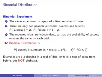
The Binomial Distribution Binomial Experiment An experiment with - PowerPoint PPT Presentation

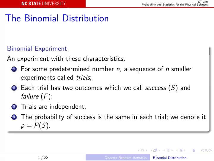
ST 380 Probability and Statistics for the Physical Sciences The Binomial Distribution Binomial Experiment An experiment with these characteristics: For some predetermined number n , a sequence of n smaller 1 experiments called trials ; Each trial has two outcomes which we call success ( S ) and 2 failure ( F ); Trials are independent; 3 The probability of success is the same in each trial; we denote it 4 p = P ( S ). 1 / 22 Discrete Random Variables Binomial Distribution

ST 380 Probability and Statistics for the Physical Sciences Examples of Binomial Experiments Toss a coin or a thumbtack a fixed number of times; S could be “heads” or “lands point up”. Sample 40 people from a large population; S could be “born in January”. Sampling Without Replacement A bowl contains 5 red M&Ms and 5 green M&Ms. Choose one at random: P (red) = 1 / 2. Without replacing it, choose another: � 4 if first was red 9 P (red) = 5 if first was green. 9 Not independent, so not a binomial experiment. 2 / 22 Discrete Random Variables Binomial Distribution

ST 380 Probability and Statistics for the Physical Sciences Binomial Random Variable X = number of successes in a binomial experiment Binomial Distribution Each outcome of a binomial experiment can be written as a string of n letters, each S or F . The sample space S is the set of all such strings. The event X = x is the subset of strings with exactly x S s, and therefore ( n − x ) F s. � n � Each such string has probability p x (1 − p ) n − x , and there are of x � n � p x (1 − p ) n − x . them, so P ( X = x ) = x 3 / 22 Discrete Random Variables Binomial Distribution

ST 380 Probability and Statistics for the Physical Sciences Shorthand: if X is a binomial random variable with n trials and success probability p , we write X ∼ B ( n , p ). The range of X is { 0 , 1 , . . . , n } . We have shown that the pmf of X , denoted b ( x ; n , p ), is � n � p x (1 − p ) n − x , b ( x ; n , p ) = P ( X = x ) = x = 0 , 1 , . . . , n . x In R n <- 10 p <- 0.25 probs <- dbinom(0:n, n, p) plot(0:n, probs, type = "h") points(0:n, probs) 4 / 22 Discrete Random Variables Binomial Distribution

ST 380 Probability and Statistics for the Physical Sciences Expected Value and Variance of X If X ∼ Bin( n , p ) and q = 1 − p , then E ( X ) = np , V ( X ) = np (1 − p ) = npq , and σ X = √ npq . Note that if n = 1, X is a Bernoulli random variable; in that case, we showed earlier that E ( X ) = p and V ( X ) = pq . 5 / 22 Discrete Random Variables Binomial Distribution

ST 380 Probability and Statistics for the Physical Sciences Hypergeometric and Negative Binomial Distributions Hypergeometric Distribution As noted earlier, sampling without replacement from a finite population is not a binomial experiment. A random sample of size n is drawn without replacement from a finite population of N items, of which M are labeled “Success” and the remaining N − M are labeled “Failure”. 6 / 22 Discrete Random Variables Hypergeometric and Negative Binomial

ST 380 Probability and Statistics for the Physical Sciences Then X , the number of successes in the sample, has the hypergeometric distribution with pmf � M �� N − M � x n − x h ( x ; n , M , N ) = � N � n for max(0 , n − N + M ) ≤ x ≤ min( n , M ). Binomial Approximation If N is much larger than n , sampling with and without replacement are roughly the same, and the hypergeometric distribution is then close to the binomial distribution: � � x ; n , M h ( x ; n , M , N ) ≈ b N 7 / 22 Discrete Random Variables Hypergeometric and Negative Binomial

ST 380 Probability and Statistics for the Physical Sciences Negative Binomial Distribution As in a binomial experiment, we carry out a sequence of independent trials, but instead of carrying out a fixed number of trials , we wait until we see a fixed number r of successes . Then X , the number of failures that occurred before stopping, has the negative binomial distribution with pmf � x + r − 1 � p r (1 − p ) x , x = 0 , 1 , 2 , . . . b neg ( x ; r , p ) = r − 1 Generalized Negative Binomial Distribution b neg ( x ; r , p ) can also be defined for non-integer r . 8 / 22 Discrete Random Variables Hypergeometric and Negative Binomial

ST 380 Probability and Statistics for the Physical Sciences The Poisson Distribution The binomial distribution, and its special case the Bernoulli distribution, are two of the most important discrete distributions. The Poisson distribution is arguably as important. Poisson distribution The random variable X has the Poisson distribution with parameter µ > 0 if its pmf is p ( x ; µ ) = e − µ µ x x ! , x = 0 , 1 , 2 , . . . 9 / 22 Discrete Random Variables Poisson Distribution

ST 380 Probability and Statistics for the Physical Sciences An Approximation The binomial distribution B ( n , p ), if n is large and p is small, is approximately the same as the Poisson distribution with parameter µ = np . To be precise, if n → ∞ and p → 0 in such a way that np → µ > 0, then b ( x ; n , p ) → p ( x ; µ ) . 10 / 22 Discrete Random Variables Poisson Distribution

ST 380 Probability and Statistics for the Physical Sciences Devore’s Rule of Thumb The approximation can safely be used when n > 50 and np < 5. What does this mean? 0 ≤ x ≤ 50 | b ( x ; 50 , 0 . 1) − p ( x , 5) | = . 0095 < . 01 max Perhaps that the difference is always less than . 01? This table shows the smallest n that achieves this for various values of µ = np . µ = np 1 2 3 4 5 6 7 8 9 10 Smallest n 19 29 36 42 48 53 58 62 66 70 11 / 22 Discrete Random Variables Poisson Distribution

ST 380 Probability and Statistics for the Physical Sciences But for large µ , all the individual probabilities are small. Perhaps we should look at the cdfs: 0 ≤ x ≤ 50 | F b ( x ; 50 , 0 . 1) − F p ( x , 5) | = . 0147 < . 015 max Perhaps the rule of thumb is that the difference in the cdfs is always less than . 015? This table shows the smallest n that achieves this for various values of µ = np . µ = np 1 3 5 7 10 15 20 25 30 40 Smallest n 13 31 50 67 95 140 183 228 271 360 12 / 22 Discrete Random Variables Poisson Distribution

ST 380 Probability and Statistics for the Physical Sciences Mean and Variance The Poisson distribution has the interesting property that both its mean and variance are equal to the parameter µ : If X has the Poisson distribution with parameter µ , then E ( X ) = V ( X ) = µ. For the binomial distribution, V ( X ) < E ( X ) , and for the negative binomial distribution, V ( X ) > E ( X ) . 13 / 22 Discrete Random Variables Poisson Distribution

ST 380 Probability and Statistics for the Physical Sciences Poisson Process The Poisson distribution is associated with the Poisson Process , which is a model for a sequence of events that occur “at random”, without memory. If the events occur in a Poisson Process with rate α (events per unit time), then the number of events in any time interval of length t has the Poisson distribution with parameter α t . The numbers of events in disjoint time intervals are statistically independent. 14 / 22 Discrete Random Variables Poisson Distribution

ST 380 Probability and Statistics for the Physical Sciences Bus Arrivals Suppose you arrive at a bus stop, waiting for a bus that runs every 20 minutes. If you know nothing about the schedule, the chance that a bus arrives in the next minute is 1 minute / 20 minute − 1 = . 05. Suppose you are told that the last bus arrived 19 minutes ago. If the buses run “on time”, the chance that a bus arrives in the next minute is now 1. But if the schedule slips, it’s less than certain. If the buses are delayed badly, the information about the last bus is irrelevant, and the buses arrive in a Poisson Process with rate 1 / 20 = 0 . 05 buses per minute. 15 / 22 Discrete Random Variables Poisson Distribution

ST 380 Probability and Statistics for the Physical Sciences Radioactive Decay A Geiger counter detects the emission of nuclear radiation, for instance from a sample of radioactive material. Emissions are generally assumed to follow a Poisson Process. 16 / 22 Discrete Random Variables Poisson Distribution

ST 380 Probability and Statistics for the Physical Sciences Probability Generating Function The probability generating function (pgf) is a useful tool for studying discrete probability distributions. If X is a discrete random variable taking non-negative integer values, its pgf is ∞ � � z X � p ( x ) z x . G ( z ) = E = x =0 17 / 22 Discrete Random Variables Probability Generating Function

ST 380 Probability and Statistics for the Physical Sciences Properties of the pgf Set z = 1: ∞ � 1 X � � G (1) = E = p ( x ) = 1 . x =0 Differentiate and set z = 1: ∞ � G ′ ( z ) = p ( x ) xz x − 1 , x =0 so ∞ � G ′ (1) = p ( x ) x = µ X . x =0 18 / 22 Discrete Random Variables Probability Generating Function

ST 380 Probability and Statistics for the Physical Sciences Binomial Distribution Suppose that X ∼ B ( n , p ); that is, X is the number of successes in n independent trials, with probability p of success in each trial. For i = 1 , 2 , . . . , n , write � 1 if trial i is a success X i = 0 if it is a failure . Then n � X = X i . i =1 19 / 22 Discrete Random Variables Probability Generating Function