Probability & Statistics: Intro, summary statistics, probability - PDF document

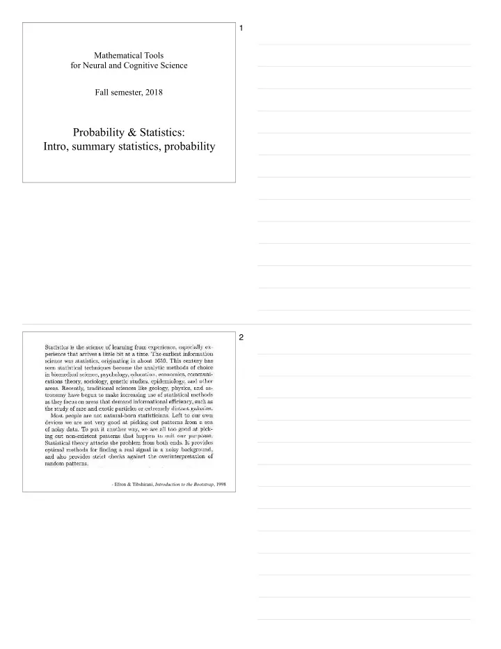
1 Mathematical Tools for Neural and Cognitive Science Fall semester, 2018 Probability & Statistics: Intro, summary statistics, probability 2 - Efron & Tibshirani, Introduction to the Bootstrap , 1998

3 Some history… • 1600’s: Early notions of data summary/averaging • 1700’s: Bayesian prob/statistics (Bayes, Laplace) • 1920’s: Frequentist statistics for science (e.g., Fisher) • 1940’s: Statistical signal analysis and communication, estimation/decision theory (e.g., Shannon, Wiener, etc) • 1950’s: Return of Bayesian statistics (e.g., Jeffreys, Wald, Savage, Jaynes…) • 1970’s: Computation, optimization, simulation (e.g,. Tukey) • 1990’s: Machine learning (large-scale computing + statistical inference + lots of data) • Since 1950’s! : statistical neural/cognitive models 4 Scientific process Observe / measure data Generate predictions, Summarize/fit model(s), design experiment compare with predictions Create/modify hypothesis/model

5 Descriptive statistics: Central tendency 6 Descriptive statistics: Central tendency • We often summarize data with the average. Why? • Average minimizes the squared error (as in regression!): N N 1 � 2 = 1 X X � µ ( ~ x ) = arg min x n − c x n N N c n =1 n =1 # 1 /p " N • Generalize: minimize L p norm: 1 | x n − c | p X arg min N c n =1 – minimize L 1 norm: median, m ( ~ x ) – minimize L 0 norm: mode – minimize norm: midpoint of range L ∞ • Issues: outliers, asymmetry, bimodality • How do we choose?


 7 Descriptive statistics: Dispersion 8 Descriptive statistics: Dispersion • Sample standard deviation 
 # 1 / 2 N " 1 X ( x n − c ) 2 � ( ~ x ) = min c N n =1 # 1 / 2 " N 1 X x )) 2 = ( x n − µ ( ~ N n =1 • Mean absolute deviation (MAD) about the median 
 N x ) = 1 X � � d ( ~ � x n − m ( ~ x ) � N n =1 • Quantiles

9 Descriptive statistics: Dispersion Summary statistics (eg: sample mean/var) can be interpreted as estimates of model parameters To formalize this, we need tools from probability… 10 probability data histogram distribution { x n } { c k , h k } p ( x )

⃗ ⃗ 11 probabilistic data model Measurement p θ ( x ) { x n } Inference 12 Probabilistic Middleville In Middleville, every family has two children, brought by the stork. The stork delivers boys and girls randomly, with family probabilistic model probability {BB,BG,GB,GG}={0.2,0.3,0.2,0.3} You pick a family at random and discover that one data of the children is a girl. What are the chances that the other child is a girl? inference

13 Statistical Middleville In Middleville, every family has two children, brought by the stork. The stork delivers boys and girls randomly, with family probability {BB,BG,GB,GG}={0.2,0.3,0.2,0.3} In a survey of 100 of the Middleville families, 32 have two girls, 23 have two boys, and the remainder one of each. You pick a family at random and discover that one data of the children is a girl. What are the chances that the other child is a girl? inference 14 Probability basics (outline) • distributions: discrete and continuous • expected value, moments • cumulative distributions. Quantiles, Q-Q plots, drawing samples. • transformations: affine, monotonic nonlinear

15 Probability: Definitions/notation Useful to have this notation up on slid, while introducing concepts on board let X , Y, Z be random variables they can take on values (like ‘heads’ or ‘tails’; or integers 1-6; or real-valued numbers) let x, y, z stand generically for values they can take, and denote events such as X = x write the probability that X takes on value x as P ( X = x ), or P X (x), or sometimes just P ( x ) P ( x ) is a function over values x, which we call the probability “distribution” function (pdf) (for continuous variables, “density”) 16 Probability distributions Discrete random variable Continuous random variable P ( x ) p ( x ) 0 < p ( x ) 0 < P ( x i ) < 1, ∀ i ∞ ∑ ∫ p ( x ) dx = 1 P ( x i ) = 1 −∞ i

17 Example distributions a not-quite-fair coin roll of a fair die sum of two rolled fair dice 0.7 0.2 0.2 0.6 0.15 0.15 0.5 0.4 0.1 0.1 0.3 0.2 0.05 0.05 0.1 0 0 0 1 2 3 4 5 6 2 3 4 5 6 7 8 9 10 11 12 0 1 clicks of a Geiger counter, horizontal velocity of gas ... and, time between clicks in a fixed time interval molecules exiting a fan 0.25 0.1 0.2 0.08 0.15 0.06 0.1 0.04 0.05 0.02 0 0 - 0 1 2 1 3 2 4 3 4 5 5 6 7 6 8 7 9 8 10 11 9 10 0 200 400 600 800 1000 18 Expected value - discrete N ∑ E ( X ) = x i p ( x i ) [the mean, ] µ i = 1 N ∑ E ( f ( X )) = More generally: f ( x i ) p ( x i ) i = 1 0.7 0.6 0.5 0.4 P(x) 0.3 0.2 0.1 0 0 1 2 3 4 # of credit cards µ

19 Expected value - continuous Z [mean, ] E ( x ) = x p ( x ) dx µ Z x 2 p ( x ) dx E ( x 2 ) = [“second moment”, m 2 ] Z ( x − µ ) 2 p ( x ) dx [variance, ] σ 2 � ( x − µ ) 2 � = E Z x 2 p ( x ) dx − µ 2 [ equal to m 2 minus ] μ 2 = Z [“expected value of f ”] E ( f ( x )) = f ( x ) p ( x ) dx Note: this is an inner product, and thus linear: E ( af ( x ) + bg ( x )) = aE ( f ( x )) + bE ( g ( x )) 20 Cumulatives 0.2 0.15 p(x) p(x) 0.1 0.05 0 50 100 150 2 3 4 5 6 7 8 9 101112 x Z y x c ( y ) = p ( x ) dx −∞ 1 1 c(x) c(x) 0.5 0 0 2 4 6 8 10 12 50 100 150 x x

21 Drawing samples - discrete 1 0.75 0.5 0.5 0.375 0.25 0.25 0.125 0 0 22 Multi-variate probability • joint distributions • marginals (integrating) • conditionals (slicing) • Bayes’ rule (inverse probability) • statistical independence (separability) • linear transformations [on board]

23 Joint and conditional probability - discrete 24 Joint and conditional probability - discrete P(Ace) P(Heart) P(Ace & Heart) “Independence” P(Ace | Heart) P(not Jack of Diamonds) P(Ace | not Jack of Diamonds)

27 Conditional probability A B A & B Neither A nor B p ( A | B ) = probability of A given that B is asserted to be true = p ( A & B ) p ( B ) 28 Conditional distribution p ( x, y ) p ( x | y = 68)

29 Conditional distribution P(x|Y=68) �Z p ( x | y = 68) = p ( x, y = 68) p ( x, y = 68) dx . = p ( x, y = 68) p ( y = 68) More generally: p ( x | y ) = p ( x, y ) /p ( y ) slice joint distribution normalize (by marginal) 30 Bayes’ Rule A B A & B p ( A | B ) = probability of A given that B is asserted to be true = p ( A & B ) p ( B ) p ( A & B ) = p ( B ) p ( A | B ) = p ( A ) p ( B | A ) ⇒ p ( A | B ) = p ( B | A ) p ( A ) p ( B )

31 Bayes’ Rule p ( x | y ) = p ( y | x ) p ( x ) /p ( y ) (a direct consequence of the definition of conditional probability) 32 Conditional vs. marginal P ( x | Y =120) P ( x ) In general, the marginals for different Y values differ. When are they they same? In particular, when are all conditionals equal to the marginal?

33 Statistical independence Random variables X and Y are statistically independent if (and only if): p ( x , y ) = p ( x ) p ( y ) ∀ x , y [note: for discrete distributions, this is an outer product!] Independence implies that all conditionals are equal to the corresponding marginal: p ( x | y ) = p ( x , y ) / p ( y ) = p ( x ) ∀ x , y 34 Sums of RVs Let Z = X + Y . Since expectation is linear: E ( X + Y ) = E ( X ) + E ( Y ) In addition, if X and Y are independent, then E ( XY ) = E ( X ) E ( Y ) ( ) = σ X ( ) 2 = E ( ) − µ X + µ Y ( ) 2 + σ Y 2 σ Z X + Y 2 and is a convolution of and p Z ( z ) p X ( x ) p Y ( y ) [on board]

35 Mean and variance • Mean and variance summarize the centroid/width • Translation and rescaling of random variables • Mean/variance of weighted sum of random variables • The sample average • ... converges to true mean (except for bizarre distributions) • ... with variance • ... most common common choice for an estimate ... 36 Central limit for a uniform distribution... 10k samples, uniform density (sigma=1) 10 4 samples of uniform dist (u+u)/sqrt(2) 250 450 400 200 350 300 150 250 200 100 150 100 50 50 0 0 − 4 − 3 − 2 − 1 0 1 2 3 4 − 4 − 3 − 2 − 1 0 1 2 3 4 (u+u+u+u)/sqrt(4) 10 u’s divided by sqrt(10) 500 600 450 500 400 350 400 300 250 300 200 200 150 100 100 50 0 0 − 4 − 3 − 2 − 1 0 1 2 3 4 − 4 − 3 − 2 − 1 0 1 2 3 4

37 Central limit for a binary distribution... one coin avg of 16 coins 6000 2000 5000 1500 4000 3000 1000 2000 500 1000 0 0 0 0.2 0.4 0.6 0.8 1 0 0.2 0.4 0.6 0.8 1 avg of 4 coins avg of 256 coins avg of 64 coins 4000 2500 2000 2000 3000 1500 1500 2000 1000 1000 1000 500 500 0 0 0 0 0.2 0.4 0.6 0.8 1 0 0 0.2 0.2 0.4 0.4 0.6 0.6 0.8 0.8 1 1