Binomial Distribution Binomial Experiment 1 The same experiment is - PowerPoint PPT Presentation

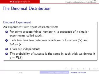
Binomial Distribution Binomial Experiment 1 The same experiment is repeated a fixed number of times. 2 There are only two possible outcomes, success and failure.; P ( success ) = p , P ( failure ) = 1 − p . 3 The repeated trials are independent, so that the probability of success remains the same for each trial. The Binomial Distribution is P ( exactly k successes in n trials) = p k (1 − p ) n − k C ( n , k ) . Examples are a 2 showing in a rool of dice, or H in a toss of coins from before, but NOT birthdays. Dan Barbasch Math 1105 Chapter 8 Week of September 17 1 / 22

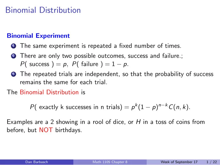
Binomial Distribution, Examples I Example (#48 Section 8.4) A hospital receives 1 / 5 = 0 . 2 of its flu vaccine shipments from Company X and the remainder of its shipments from other companies. Each shipment contains a very large number of vaccine vials. For Company X’s shipments, 10% of the vials are ineffective. For every other company, 2% of the vials are ineffective. The hospital tests 30 randomly selected vials from a shipment and finds that one vial is ineffective. What is the prob- ability that this shipment came from Company X? Dan Barbasch Math 1105 Chapter 8 Week of September 17 2 / 22

Binomial Distribution, Examples II Answer. For X , p = 0 . 1 and 1 − p = 0 . 9, for NX , p = 0 . 02 and 1 − p = 0 . 98 . P ( X ) = 0 . 2 P ( NX ) = 0 . 8 P ( D | X ) = 0 . 1 P ( D | NX ) = 0 . 02 P (1 D / 30 | X ) = C (30 , 1) × (0 . 1) 1 × (0 . 9) 29 P (1 D / 30 | NX ) = C (30 , 1) × (0 . 02) 1 × (0 . 98) 29 Draw the usual tree diagram for Bayes’s theorem and compute. P ( X | 1 D / 30) = P (1 D / 30 and X ) = P (1 D / 30) C (30 , 1) · (0 . 1) 1 · (0 . 9) 29 · 0 . 2 = C (30 , 1) · (0 . 1) 1 · (0 . 9) 29 · 0 . 2 + C (30 , 1) · (0 . 02) 1 · (0 . 98) 29 · 0 . 8 . The answer is (close to) 0 . 1. Dan Barbasch Math 1105 Chapter 8 Week of September 17 3 / 22

Pascal’s Triangle I The triangular array of numbers shown below is called Pascals triangle in honor of the French mathematician Blaise Pascal (1623 - 1662), who was one of the first to use it extensively. The triangle was known long before Pascals time and appears in Chinese and Islamic manuscripts from the eleventh century. 1 1 1 1 2 1 1 3 3 1 1 4 6 4 1 1 5 10 10 5 1 The array provides a quick way to find binomial probabilities. The n th row of the triangle, where n = 0 , 1 , 2 , 3 , . . . , gives the coefficients C ( n , r ) for r = 0 , 1 , 2 , 3 , . . . , n . For example, for n = 4, 1 = C (4 , 0) , 4 = C (4 , 1) , 6 = C (4 , 2), and so on. Each number in the Dan Barbasch Math 1105 Chapter 8 Week of September 17 4 / 22

Pascal’s Triangle II triangle is the sum of the two numbers directly above it. For example, in the row for n = 4 , 1 is the sum of 1 , the only number above it, 4 is the sum 1 + 3, 6 = 3 + 3 and so on. The general formula is C ( n , r ) = C ( n − 1 , r − 1) + C ( n − 1 , r ) . Choosing r out of n is the same as the sum of choose r out of n − 1 (make the choice of all r out of 1 , . . . , n − 1 plus choose r − 1 out of n − 1 (choose n and then r − 1 out of n − 1). Dan Barbasch Math 1105 Chapter 8 Week of September 17 5 / 22

Example, Sports I In many sports championships, such as the World Series in baseball and the Stanley Cup final series in hockey, the winner is the first team to win four games. For this exercise, assume that each game is independent of the others, with a constant probability p that one specified team (say, the National League team) wins. a. Find the probability that the series lasts for four, five, six, and seven games when p = 0 . 5. b. Morrison and Schmittlein have found that the Stanley Cup finals can be described by letting p = 0 . 73 be the probability that the better team wins each game. Find the probability that the series lasts for four, five, six, and seven games. Source: Chance . Dan Barbasch Math 1105 Chapter 8 Week of September 17 6 / 22

Example, Sports II Answer. P ( End in exactly 4 ) = P ( AAAA and BBBB } = 2 · (0 . 5) 4 , P ( End in exactly 5 ) = C (4 , 1)(0 . 5) 5 + C (4 , 3)(0 . 5) 5 , P ( End in exactly 6 ) = C (5 , 2) · (0 . 5) 6 + C (5 , 3)(0 . 5) 6 , P ( End in exactly 7 ) = C (6 , 3)(0 . 5) 7 + C (6 , 3)(0 . 5) 7 . From the triangle, C (4 , 1) = C (3 , 1) + C (3 , 0) = 3 + 1 = 4 , C (4 , 3) = C (3 , 3) + C (3 , 2) = 1 + 3 = 4 , C (5 , 2) = C (4 , 2) + C (4 , 1) = 6 + 4 = 10 , C (5 , 3) = C (4 , 3) + C (4 , 2) = 4 + 6 = 10 , C (6 , 3) = C (5 , 3) + C (5 , 2) = 10 + 10 = 20 . Dan Barbasch Math 1105 Chapter 8 Week of September 17 7 / 22

Fermat and Pascal I Fand P are playing a game. They toss a coin, p = P ( H ) = 0 . 3 . F wins if H , P wins if T . F leads 8 to 7. What is the probability that the game ends whenever one reaches 20. What is the probability the game ends after another 1 12 2 20 tosses? Dan Barbasch Math 1105 Chapter 8 Week of September 17 8 / 22

Fermat and Pascal II Answer. For (1), p 12 . Only F can win. For (2) C (19 , 12) p 12 (1 − p ) 8 + C (19 , 13) p 7 (1 − p ) 13 . The sum of probabilities that F wins and that P wins. Dan Barbasch Math 1105 Chapter 8 Week of September 17 9 / 22

Random Variables I Random Variable A random variable X is a function that assigns a real number to each outcome of an experiment. Probability Distribution The probability distribution of a radom variable is { P ( X = k ) = p k } with 0 ≤ p k ≤ 1 and the sum of p k , � n k =0 = 1 . This definition is for when X takes finitely many values only. Expected Value E ( X ) = � k kP ( X = k ) . Example Toss a coin. Let X = 1 if H , and X = 0 if T . The coin satisfies P ( H ) = p and P ( T ) = 1 − p . The probability distribution is P ( X = 1) = 1 and P ( X = 0) = 1 − p . Then EX = 1 · p + 0 · (1 − p ) = p . If X = 1 if H , and X = − 1 if T , then EX = 1 · p + ( − 1) · (1 − p ) = 2 p − 1 . Dan Barbasch Math 1105 Chapter 8 Week of September 17 10 / 22

Random Variables II Example Toss two fair dice. Let X be the sum of the faces. P ( X = 2) = 1 / 36 P ( X = 3) = 2 / 36 P ( X = 4) = 3 / 36 P ( X = 5) = 4 / 36 P ( X = 6) = 5 / 36 P ( X = 7) = 6 / 36 P ( X = 8) = 5 / 36 P ( X = 9) = 4 / 36 P ( X = 10) = 3 / 36 P ( X = 11) = 2 / 36 P ( X = 12) = 1 / 36 Then EX = 2 · 1 / 36 + 3 · 2 / 36 + 4 · 3 / 36 + 5 · 4 / 36 + 6 · 5 / 36 + 7 · 6 / 36 + 8 · 5 / 36 + 9 · 4 / 36 + 10 · 3 / 36 + 11 · 2 / 36 + 12 · 1 / 36= 7 . Dan Barbasch Math 1105 Chapter 8 Week of September 17 11 / 22

Motivation Suppose you have a coin that comes up H 30% of times and T 70% of times. You get paid $2 if H, and you pay out $1 if T. What do you expect to have after 100 tosses? The intuition says it should be the average, 2 · 30 − 1 · 70 = − 10. For one toss you’d expect 2 · 0 . 3 + ( − 1) · 0 . 7 = − 0 . 1. Repeat a 100 times, and you expect to have lost $10. The mathematics is the Expected Value. We interpret P ( H ) = 0 . 3 and P ( T ) = 0 . 7 . The expected value is EX = 2 · P ( H ) + ( − 1) · P ( T ). For n tosses you expect nEX . Dan Barbasch Math 1105 Chapter 8 Week of September 17 12 / 22

Expected Value of a Sum of Independent Variables I Definition Two random variables X 1 , X 2 are called independent if P ( X 1 = a , X 2 = b ) = P ( X 1 = a ) · P ( X 2 = b ). More general, X 1 , . . . X n are called independent if P ( X i 1 = a 1 , . . . X i k = a k ) = P ( X i 1 = i 1 ) · P ( X i k = a k ) for any choice of a subset of the variables. Theorem Let X 1 , . . . , X n be independent random variables. Then E ( X 1 + · · · + X n ) = EX 1 + · · · + EX n We ilustrate the proof for the case n = 2 , E ( X 1 + X 2 ) = EX 1 + EX 2 . This is the warmup. P ( X 1 = a 1 ) = p P ( X 1 = a 2 ) = 1 − p P ( X 2 = b 1 ) = q P ( X 2 = b 2 ) = 1 − q . Dan Barbasch Math 1105 Chapter 8 Week of September 17 13 / 22

Expected Value of a Sum of Independent Variables II EX 1 = a 1 p + a 2 (1 − p ) EX 2 = b 1 q + b 2 (1 − q ) E ( X 1 + X 2 ) = ( a 1 + b 1 ) pq + ( a 1 + b 2 ) p (1 − q )+ ( a 2 + b 1 )(1 − p ) q + ( a 2 + b 2 )(1 − p )(1 − q ) Gather the terms according to the a ′ s and b ′ s , and do the algebra. a 1 ( pq + p (1 − q )) = a 1 p a 2 ((1 − p ) q + (1 − p )(1 − q )) = a 2 (1 − p ) b 1 ((1 − p ) q + pq ) = b 1 q b 2 ( p (1 − q ) + 1 − p )(1 − q )) = b 2 (1 − q ) . Dan Barbasch Math 1105 Chapter 8 Week of September 17 14 / 22

Expected Value of a Sum of Independent Variables III Example (Binomial distribution) For n independent identical trials each with two possible outcomes, S and F, with probability p and 1 − p , X the number of S , the distribution is P ( X = k ) = C ( n , k ) p k (1 − p ) n − k . The expected value is n � kC ( n , k ) p k (1 − p ) n − k = np . EX = k =0 For a single trial, EX = p · 1 + 0 · (1 − p ) = p . The general case can be computed directly using algebra. Dan Barbasch Math 1105 Chapter 8 Week of September 17 15 / 22

Binomial Distribution We apply this to the binomial distribution, X 1 , . . . , X n i.i.d. (independent identically distributed random variables) with probability distribution P ( X = 1) = p , P ( X = 0) = 1 − p . Then EX = 1 · p + 0 · (1 − p ) = p . So E ( X 1 + · · · + X n ) = p + · · · + p = np . � �� � n The case of two dice is similar; X = X 1 + X 2 . Then EX 1 = EX 2 = 1 · 1 / 6+2 · 1 / 6+3 · 1 / 6+4 · 1 / 6+5 · 1 / 6+6 · 1 / 6 = 21 / 6 = 7 / 2 . So E ( X 1 + X 2 ) = 7 / 2 + 7 / 2 = 7. Dan Barbasch Math 1105 Chapter 8 Week of September 17 16 / 22