1.10.2 Normal distribution 1.10.3 Approximating binomial - PowerPoint PPT Presentation

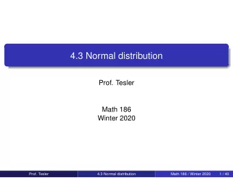
1.10.2 Normal distribution 1.10.3 Approximating binomial distribution by normal 2.10 Central Limit Theorem Prof. Tesler Math 283 Fall 2019 Prof. Tesler 1.10.2-3, 2.10 Normal distribution Math 283 / Fall 2019 1 / 38

Normal distribution a.k.a. “Bell curve” and “Gaussian distribution” The normal distribution is a continuous distribution. Parameters: µ = mean (center) σ = standard deviation (width) � − ( x − µ ) 2 � 1 PDF: f X ( x ) = 2 π exp for − ∞ < x < ∞ . 2 σ 2 √ σ Normal distribution N ( 20 , 5 ) : µ = 20, σ = 5 0.08 Normal µ µ ± σ 0.04 pdf 0.00 0 10 20 30 40 x The normal distribution is symmetric about x = µ , so median = mean = µ . Prof. Tesler 1.10.2-3, 2.10 Normal distribution Math 283 / Fall 2019 2 / 38

Applications of normal distribution Applications Coverage in DNA sequencing Many natural quantities are modelled by it: e.g., a Illumina GA II sequencing of histogram of the heights or E. coli at 600 × coverage. weights of everyone in a large Chitsaz et al. (2011), Nature Biotechnology population often follows a Empirical distribution of coverage normal distribution. 1.0 Many distributions such as % of positions with coverage 0.8 binomial, Poisson,... are 0.6 closely approximated by it when the parameters are large 0.4 enough. 0.2 Sums and averages of huge 0.0 quantities of data are often 0 200 400 600 800 1000 modelled by it. Coverage Prof. Tesler 1.10.2-3, 2.10 Normal distribution Math 283 / Fall 2019 3 / 38

Cumulative distribution function The cumulative distribution function is the integral � x −( t − µ ) 2 � � 1 √ exp F X ( x ) = P ( X � x ) = dt 2 σ 2 σ 2 π − ∞ The usual strategy to compute integrals is antiderivatives, like � x 2 dx = x 3 3 + C . But this doesn’t have an antiderivative in terms of the usual functions (polynomials, exponentials, logs, trig, . . . ). The integral can be done via numerical integration or Taylor series. The integral for total probability equals 1; this can be shown using double integrals in polar coordinates: � ∞ −( x − µ ) 2 � � 1 √ exp dx = 1 2 σ 2 σ 2 π − ∞ Prof. Tesler 1.10.2-3, 2.10 Normal distribution Math 283 / Fall 2019 4 / 38

Standard normal distribution Standard normal distribution N ( 0 , 1 ) : µ = 0, σ = 1 CDF of standard normal distribution 0.4 Normal Normal µ µ µ 0.8 µ ± σ µ µ ± σ pdf 0.2 cdf 0.4 0.0 0.0 −4 −2 0 2 4 −4 −2 0 2 4 z z The standard normal distribution is the normal distribution for µ = 0 , σ = 1 . Use the variable name Z : φ ( z ) = f Z ( z ) = e − z 2 / 2 PDF: for − ∞ < z < ∞ √ 2 π � z 1 e − t 2 / 2 dt √ CDF: Φ ( z ) = F Z ( z ) = P ( Z � z ) = 2 π − ∞ The integral requires numerical methods. In the past, people used lookup tables. We’ll use functions for it in Matlab and R. Prof. Tesler 1.10.2-3, 2.10 Normal distribution Math 283 / Fall 2019 5 / 38

Matlab and R commands For the standard normal: Φ − 1 ( . 9750 ) ≈ 1 . 96 Φ ( 1 . 96 ) ≈ 0 . 9750 Matlab: normcdf ( 1 . 96 ) norminv ( . 9750 ) R: pnorm ( 1 . 96 ) qnorm(.9750) We will see shortly how to convert between an arbitrary normal distribution (any µ , σ ) and the standard normal distribution. The commands above allow additional arguments to specify µ and σ , e.g., normcdf(1.96,0,1) . R also can work with the right tail directly: pnorm ( 1 . 96 , lower . tail = FALSE ) ≈ 0 . 9750 qnorm ( 0 . 9750 , lower . tail = FALSE ) ≈ 1 . 96 Prof. Tesler 1.10.2-3, 2.10 Normal distribution Math 283 / Fall 2019 6 / 38

Standard normal distribution — areas Standard Normal Curve 0.4 0.3 pdf 0.2 0.1 0 ! 5 a 0 b 5 z The area between z = a and z = b is � b 1 e − t 2 / 2 dt = Φ ( b ) − Φ ( a ) √ P ( a � Z � b ) = 2 π a P ( 1 . 51 � Z � 1 . 62 ) = Φ ( 1 . 62 ) − Φ ( 1 . 51 ) = 0 . 9474 − 0 . 9345 = 0 . 0129 Matlab: normcdf ( 1 . 62 ) − normcdf ( 1 . 51 ) R: pnorm ( 1 . 62 ) − pnorm ( 1 . 51 ) Prof. Tesler 1.10.2-3, 2.10 Normal distribution Math 283 / Fall 2019 7 / 38

Standard normal distribution — symmetries of areas Area ! on the right &'()* ! *+,*-.(*/(0- 0.4 "#$ pdf 120 0.2 "#! z ! ! % ! 0 " ! 2 0 2 ! ! " ! z % Area right of z is P ( Z > z ) = 1 − Φ ( z ) . By symmetry, the area left of − z and the area right of z are equal: Φ (− z ) = 1 − Φ ( z ) Φ (− 1 . 51 ) = 1 − Φ ( 1 . 51 ) = 1 − 0 . 9345 = 0 . 0655 Area between z = ± a : Φ ( a ) − Φ (− a ) = Φ ( a ) − ( 1 − Φ ( a )) = 2 Φ ( a ) − 1 Φ ( 1 . 51 ) − Φ (− 1 . 51 ) = 2 Φ ( 1 . 51 ) − 1 ≈ . 8690 Prof. Tesler 1.10.2-3, 2.10 Normal distribution Math 283 / Fall 2019 8 / 38

Central area Area ! split half on each tail 0.4 Area between z = ± 1 is ≈ 68 . 27 %. pdf Area between z = ± 2 is ≈ 95 . 45 %. 0.2 Area between z = ± 3 is ≈ 99 . 73 %. ! z ! /2 z ! /2 0 ! 2 0 2 z Find the center part containing 95 % of the area Put 2 . 5 % of the area at the upper tail, 2 . 5 % at the lower tail, and 95 % in the middle. The value of z putting 2 . 5 % at the top gives Φ ( z ) = 1 − 0 . 025 = 0 . 975 . Notation: z . 025 = 1 . 96 . The area between z = ± 1 . 96 is about 95 %. For 99 % in the middle, 0 . 5 % on each side, use z . 005 ≈ 2 . 58 . Prof. Tesler 1.10.2-3, 2.10 Normal distribution Math 283 / Fall 2019 9 / 38

Areas on normal curve for arbitrary µ , σ � b −( x − µ ) 2 � � 1 √ P ( a � X � b ) = exp dx 2 σ 2 σ 2 π a Substitute z = x − µ (or x = σ z + µ ) into the x integral to turn it into σ the standard normal integral: � a − µ � � a − µ � � X − µ � b − µ � Z � b − µ = P P σ σ σ σ σ � b − µ � � a − µ � = Φ − Φ σ σ The z -score of x is z = x − µ σ . Prof. Tesler 1.10.2-3, 2.10 Normal distribution Math 283 / Fall 2019 10 / 38

Binomial distribution Compute P ( 43 � X � 51 ) when n = 60 , p = 3 / 4 Binomial: n = 60 , p = 3 / 4 Mean µ = np = 60 ( 3 / 4 ) = 45 � 60 ( . 75 ) k ( . 25 ) 60 − k � P ( X = k ) = k k Standard deviation 0 . 09562 43 � 0 . 11083 44 σ = np ( 1 − p ) 0 . 11822 45 � = 60 ( 3 / 4 )( 1 / 4 ) √ 0 . 11565 46 = 11 . 25 ≈ 3 . 354101966 0 . 10335 47 Mode ( k with max pdf) 0 . 08397 48 0 . 06169 49 ⌊ np + p ⌋ 0 . 04071 50 = ⌊ 60 ( 3 / 4 ) + ( 3 / 4 ) ⌋ 0 . 02395 51 � 45 3 � = = 45 4 Total 0 . 75404 Prof. Tesler 1.10.2-3, 2.10 Normal distribution Math 283 / Fall 2019 11 / 38

Mode of a distribution The mode of random variable X is the value k at which the pdf is maximum. Mode of binomial distribution when 0 < p < 1 The mode is ⌊ ( n + 1 ) p ⌋ . Exception: If ( n + 1 ) p is an integer then ( n + 1 ) p and ( n + 1 ) p − 1 are tied as the mode. The mode is within 1 of the mean np . When np is an integer, the mode equals the mean. Prof. Tesler 1.10.2-3, 2.10 Normal distribution Math 283 / Fall 2019 12 / 38

Binomial and normal distributions Normal approximation to binomial Binomial Binomial: n=60, p=3/4 0.15 P ( X = k ) k Binomial P(43 ! X ! 51) 0 . 09562 43 Normal: µ =45, " =3.35 0 . 11083 44 0.1 0 . 11822 45 pdf 0 . 11565 46 0 . 10335 47 0 . 08397 48 0.05 0 . 06169 49 0 . 04071 50 0 . 02395 51 0 41 43 45 47 49 51 53 55 Total 0 . 75404 x P ( X = k ) is shown as a rectangle centered above X = k : Height P ( X = k ) . Extent k ± 1 / 2 gives width 1. Area 1 · P ( X = k ) = P ( X = k ) . Area of all purple rectangles is P ( 43 � X � 51 ) . Prof. Tesler 1.10.2-3, 2.10 Normal distribution Math 283 / Fall 2019 13 / 38

Binomial and normal distributions Normal approximation to binomial Binomial Binomial: n=60, p=3/4 0.15 P ( X = k ) k Binomial P(43 ! X ! 51) 0 . 09562 43 Normal: µ =45, " =3.35 0 . 11083 44 0.1 0 . 11822 45 pdf 0 . 11565 46 0 . 10335 47 0 . 08397 48 0.05 0 . 06169 49 0 . 04071 50 0 . 02395 51 0 41 43 45 47 49 51 53 55 Total 0 . 75404 x The binomial distribution is only defined at the integers, and is very close to the normal distribution shown. We will approximate the probability P ( 43 � X � 51 ) we had above by the corresponding one for the normal distribution. Riemann sums in Calculus: area under curve ≈ area of rectangles Prof. Tesler 1.10.2-3, 2.10 Normal distribution Math 283 / Fall 2019 14 / 38

Normal approximation to binomial, step 1 Compute corresponding parameters We want to approximate P ( a � X � b ) in a binomial distribution. We’ll use n = 60 , p = 3 / 4 and approximate P ( 43 � X � 51 ) . Determine µ , σ : µ = np = 60 ( 3 / 4 ) = 45 √ � 11 . 25 ≈ 3 . 354 σ = np ( 1 − p ) = The normal distribution with those same values of µ , σ is a good approximation to the binomial distribution provided µ ± 3 σ are both between 0 and n . Check: µ − 3 σ ≈ 45 − 3 ( 3 . 354 ) = 34 . 938 µ + 3 σ ≈ 45 + 3 ( 3 . 354 ) = 55 . 062 are both between 0 and 60 , so we may proceed. Note: Some applications are more strict and may require µ ± 5 σ or more to be between 0 and n . Since µ + 5 σ ≈ 61 . 771 , this would fail at that level of strictness. Prof. Tesler 1.10.2-3, 2.10 Normal distribution Math 283 / Fall 2019 15 / 38