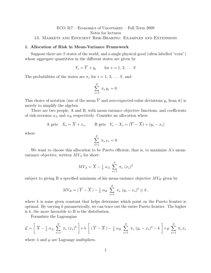
ECO 317 Economics of Uncertainty Fall Term 2009 Notes for lectures - PDF document

ECO 317 – Economics of Uncertainty – Fall Term 2009 Notes for lectures 13. Markets and Efficient Risk-Bearing: Examples and Extensions 1. Allocation of Risk in Mean-Variance Framework Suppose there are S states of the world, and a single physical good (often labelled “corn”) whose aggregate quantitites in the different states are given by Y s = Y + y s for s = 1, 2, . . . S The probabilities of the states are π s for s = 1, 2, . . . S , and S � π s y s = 0 s =1 This choice of notation (use of the mean Y and zero-expected-value deviations y s from it) is merely to simplify the algebra. There are two people, A and B, with mean-variance objective functions, and coefficients of risk-aversion α A and α B respectively. Consider an allocation where A gets X s = X + x s , B gets Y s − X s = ( Y − X ) + ( y s − x s ) where S � π s x s = 0 s =1 We want to choose this allocation to be Pareto efficient, that is, to maximize A’s mean- variance objective, written MV A for short: S MV A = X − 1 � π s ( x s ) 2 2 α A s =1 subject to giving B a specified minimum of his mean-variance objective MV B given by S π s ( y s − x s ) 2 ≥ k , MV B = ( Y − X ) − 1 � 2 α B s =1 where k is some given constant that helps determine which point on the Pareto frontier is optimal. By varying k parametrically, we can trace out the entire Pareto frontier. The higher is k , the more favorable to B is the distribution. Formulate the Lagrangian � S � � S � S π s ( y s − x s ) 2 − k X − 1 � π s ( x s ) 2 ( Y − X ) − 1 � � L = 2 α A + λ 2 α B + µ π s x s s =1 s =1 s =1 where λ and µ are Lagrange multipliers. 1

If the maximization occurs in the interior of the range of X , we have the first-order condition for X : ∂ L ∂X = 1 − λ = 0 . I will assume this to be so. There will be upper and lower limits on X implied by the requirement that the consumption quantities of both A and B must be non-negative in every state s , but I will not pursue this here. With λ = 1, the Lagrangian simplifies to S S S π s ( x s ) 2 − 1 π s ( y s − x s ) 2 − k + µ � � � L = Y − 1 2 α A 2 α B π s x s . s =1 s =1 s =1 Note that X cancels, so its exact choice is actually indeterminate. Varying k over its per- missible range changes X over its permissible range and traces out the entire set of Pareto efficient allocations. The first-order condition with respect to any one of the x s , say x σ , is ∂ L = − α A π σ x σ + α B π σ ( y σ − x σ ) + µ π σ = 0 ∂x σ Summing these over σ and using the conditions that the expected deviations are zero and that the probabilities sum to 1, we have − α A ∗ 0 + α B ∗ 0 + µ ∗ 1 = 0 or µ = 0. (A Lagrange multiplier being zero is unusual but not impossible; it means that a slight shift of the constraint has no first-order effect, but only a second-order effect, on the maximized value of the objective function.) Then the first-order conditions become − α A π σ x σ + α B π σ ( y σ − x σ ) = 0 They yield the solution α B x σ = y σ α A + α b and therefore α A y σ − x σ = y σ α A + α b for all states of the world σ = 1, 2, . . . S . In words, the shares of the two people in the deviations of aggregate output from its mean should be inversely proportional to their coefficients of risk-aversion (or equivalently, proportional to the coefficients of risk-tolerance; see the textbook, pp.153-5, also a more general formulation on pp.161-3). This makes good intuitive sense. In particular, note that if one of the two people is risk-neutral, he should bear all the risk, giving the other a constant amount across all states. The simplicity of the formula comes from the mean-variance assumption. Recall that under this assumption the absolute amount of risk a person wants to take is independent 2

of his initial wealth (similar to the case of zero income effects under quasilinear utility functions in the theory of consumer choice without uncertainty). That is why the risk- bearing optimum depends only on the risk aversion coefficients and not on the two people’s wealth levels (or on the parameter k that governs where on the Pareto frontier the two will be located). In particular, the allocation of risk is determinate, and the same at all Pareto efficient allocations, independently of whether A or B is overall better off. Again this is because the willingness of each to bear risk is independent of the extent of his well-being. To justify the mean-variance structure rigorously, we should assume that the traders have CARA utility-of-consequences functions and that the random output has a normal distribution. To do this mathematically rigorously would require a continuum of states, and therefore a constrained optimization problem where one chooses a whole function x ( s ) using the calculus of variations (isoperimetric problem). This can be done, but the discrete formulation here is simpler to explain; think of it as an approximation to the normal. In later topics we will come across situations where unobservable actions of one person can affect the overall outcome (moral hazard). Then to give this person a stronger incentive to take the socially efficient action, we will have to inflict more of risk on him than is indicated by the above formula. In other words, the optimum will have to strike a balance between the considerations of risk-bearing and incentive. Keep in mind the above formula as a reference point or standard with which to compare these later optima under moral hazard. In this section we did not consider markets where people could trade voluntarily. Instead the focus was on the Pareto frontier, where a government or some such agency reallocated quantities. But we know from the Arrow-Debreu theory of general equilibrium under uncer- tainty that any Pareto efficient allocation can be achieved as an equilibrium of price-taking trading in a complete set of Arrow-Debreu securities (or equivalently, any set of securities whose payoff vectors span the full state space) provided the initial purchasing power is suit- ably distributed. 2. Incomplete Markets – Example What happens if a complete set of Arrow-Debreu securities (or a set of fully spanning securities) is not available? Here we develop the ideas using an example, and focusing on efficient allocations. In the next section we will consider the relation between efficient allocations and equilibria of price-taking trade in markets in the available limited set of securities. Suppose there is one physical good, corn. There are two farmers, A and B. Each is subject to risk, and with equal probability may get a high output or a low output. Their risks are independent of each other. A’s high output is 30 and low output is 10 (mean 20 with equiprobable deviations of 10 on each side of the mean), whereas B’s high output is 40 and low output is 0 (mean 20 with equiprobable deviations of 20 on each side). Thus they have equal expected levels of output ( µ A = µ B = 20) but B faces more risk (variance σ 2 B = 400 as against A’s σ 2 A = 100). Suppose each has a mean-variance objective function, with µ A − 1 5 σ 2 MV A = A 20 σ 2 µ B − 1 MV B = B 3

Thus A has a coefficient of absolute risk aversion α A = 2 1 5 , whereas B has α B = 10 . Without any trade in risk, the values of the objective functions for the two people are 20 − 1 MV A = 5 100 = 0 20 − 1 MV B = 20 400 = 0 There is nothing special about these zeroes; we could have added any constant to each objective function, or multiplied it by any positive constant (taken any affine transformation of each) without affecting anything. But the zeroes are easier to remember and compare against alternatives we will consider. Specifically, we will ask how the two can trade risks for mutual benefit. We know from the general theory that price-taking trading with complete markets in Arrow-Debreu securities achieves a Pareto efficient allocation of risk. Let us consider fully efficient allocations in detail for this example. In Arrow-Debreu terms, there are four states of the world, counting all possible combi- nations of high and low outputs for the two people. Label these by two-letter combinations, the first showing A’s high or low outcome and the second showing B’s high or low. The aggregate output quantities are HH: 70; LH :50; HL: 30; LL :10 The probability of each state is 1 4 . Using the terminology of the previous section, the mean aggregate output is Y = 40, and the deviations from the mean in the four states are respec- tively 30, 10, − 10 and − 30. We know how to characterize the Pareto frontier from the general theory of the previous section. The deviations should be allocated between A and B in inverse proportions of their coefficients of absolute risk aversion, that is, 1:4. So A’s deviations from his mean should be 6, 2, − 2 and − 6, and B’s should be 24, 8, − 8 and − 24. The distributional considerations are optimally handled by giving A the average X and giving B the average 40 − X . The Pareto frontier is traced out by varying X . With these deviations, the variance of A’s final consumption of corn is 4 [ 6 2 + 2 2 + ( − 2) 2 + ( − 6) 2 ] = 1 1 4 [36 + 4 + 4 + 36] = 20 and therefore A’s mean-variance objective is MV A = X − 1 5 20 = X − 4 . The variance of B’s final consumption of corn is 4 [ 24 2 + 8 2 + ( − 8) 2 + ( − 24) 2 ] = 1 1 4 [576 + 64 + 64 + 576] = 320 and therefore B’s mean-variance objective is MV B = 40 − X − 1 20 320 = 40 − X − 16 = 24 − X . 4