ECO 317 Economics of Uncertainty Fall Term 2009 Tuesday October 6 - PowerPoint PPT Presentation

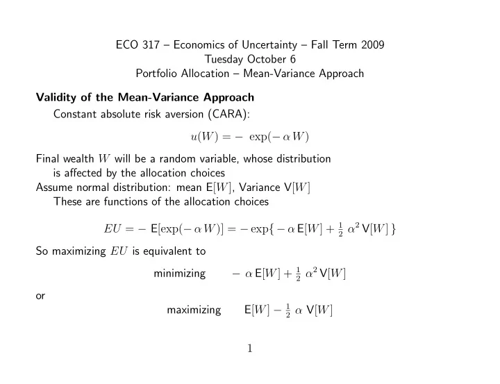
ECO 317 – Economics of Uncertainty – Fall Term 2009 Tuesday October 6 Portfolio Allocation – Mean-Variance Approach Validity of the Mean-Variance Approach Constant absolute risk aversion (CARA): u ( W ) = − exp( − α W ) Final wealth W will be a random variable, whose distribution is affected by the allocation choices Assume normal distribution: mean E [ W ] , Variance V [ W ] These are functions of the allocation choices 2 α 2 V [ W ] } EU = − E [exp( − α W )] = − exp { − α E [ W ] + 1 So maximizing EU is equivalent to 2 α 2 V [ W ] − α E [ W ] + 1 minimizing or E [ W ] − 1 maximizing 2 α V [ W ] 1

One Riskless, One Risky Asset Safe asset: gross return rate R (1 plus interest rate) Risky asset: random gross return rate r Mean µ = E [ r ] > R , Variance σ 2 = V [ r ] Initial wealth W 0 . If x in risky asset, final wealth W = ( W 0 − x ) R + x r = R W 0 + ( r − R ) x E [ W ] = W 0 R + x ( µ − R ) x 2 σ 2 ; V [ W ] = Std. Dev. = x σ 2 α x 2 σ 2 Choose x to maximize W 0 R + x ( µ − R ) − 1 FOC µ − R − a x σ 2 = 0 , therefore optimum x = µ − R α σ 2 Observe x independent of W 0 . CARA-Normal model under uncertainty is like quasi-linear utility in ordinary demand theory. 2

As x varies, straight line in (Mean,Std.Dev.) figure. expected wealth P r P* P s standard deviation P s = (0 , W 0 R ) safe; P r = ( W 0 σ, W 0 µ ) risky; Beyond P r possible if leveraged borrowing OK (In dotted line as shown if borrowing rate = safe rate R ; with kink if borrowing rate > safe rate.) P ∗ is optimal portfolio 3

Two Risky Assets W 0 = 1 ; Random gross return rates r 1 , r 2 Means µ 1 > µ 2 ; Std. Devs. σ 1 , σ 2 , Correl. Coefft. ρ Portfolio ( x, 1 − x ) . Final W = x r 1 + (1 − x ) r 2 E [ W ] = x µ 1 + (1 − x ) µ 2 = µ 2 + x ( µ 1 − µ 2 ) x 2 ( σ 1 ) 2 + (1 − x ) 2 ( σ 2 ) 2 + 2 x (1 − x ) ρ σ 1 σ 2 V [ W ] = ( σ 2 ) 2 − 2 x [ ( σ 2 ) 2 − ρ σ 1 σ 2 ] + x 2 [( σ 1 ) 2 − 2 ρ σ 1 σ 2 + ( σ 2 ) 2 ] = − 2 [( σ 2 ) 2 − ρ σ 1 σ 2 ]  at x = 0 ∂ V [ W ]  = 2 [( σ 1 ) 2 − ρ σ 1 σ 2 ] ∂x at x = 1  So diversification can reduce variance if ρ < min [ σ 1 /σ 2 , σ 2 /σ 1 ] ( σ 2 ) 2 − ρ σ 1 σ 2 To minimize variance, x = ( σ 1 ) 2 − 2 ρ σ 1 σ 2 + ( σ 2 ) 2 4

µ 1 − µ 2 + ( σ 2 ) 2 − ρ σ 1 σ 2 α Optimum: x = ( σ 1 ) 2 − 2 ρ σ 1 σ 2 + ( σ 2 ) 2 expected wealth P* P 1 P m P 2 standard deviation P 1 , P 2 points for each asset; P m minimum-variance portfolio, P ∗ optimum Portion P 2 P m dominated; P m P 1 efficient frontier Continuation past P 1 if short sales of 2 OK 5

One Riskless, Two Risky Assets First combine two riskies; this gets all points like P h on all lines like P s P r Then mix with riskless; this gets Efficient frontier P s P F tangential to risky combination curve expected wealth P 1 P P* F P r P Ph P m s P 2 standard deviation Then along curve segment P F P 1 if no leveraged borrowing; continue straight line P s P F if leveraged borrowing OK 6

With preferences as shown, optimum P ∗ mixes safe asset with particular risky combination P F “Mutual fund” P F is the same for all investors regardless of risk-aversion (so long as optimum in P s P F ) Investors who are even less risk-averse may go beyond P F including corner solution at P 1 or tangency past P 1 if can sell 2 short to buy more 1 7

Capital Asset Pricing Model Individual investors take the rates of return as given but these must be determined in equilibrium Suppose one safe and two risky assets Investor h with initial wealth W h Invests x h 1 dollars in the shares of firm 1, x h 2 dollars in the shares of firm 2, and ( W h − x h 1 − x h 2 ) in the safe asset. Expression for random final wealth W = ( W h − x h 1 − x h 2 ) R + x h 1 r 1 + x h 2 r 2 = W h R + x h 1 ( r 1 − R ) + x h 2 ( r 2 − R ) , Maximizes E [ W ] − 1 2 α h V [ W ] where W h R + x h 1 ( E [ r 1 ] − R ) + x h E [ W ] = 2 ( E [ r 2 ] − R ) 1 ) 2 V [ r 1 ] + 2 x h 2 ) 2 V [ r 2 ] ( x h 1 x h 2 Cov [ r 1 , r 2 ] + ( x h V [ W ] = 8

FOCs for optimal portfolio choice (allowing short sales etc. if necessary) α h { x h 1 V [ r 1 ] + x h E [ r 1 ] − R = 2 Cov [ r 1 , r 2 ] } α h { x h 1 Cov [ r 1 , r 2 ] + x h E [ r 2 ] − R = 2 V [ r 2 ] } like “inverse demand functions”. Rewrite these equations as x h 1 V [ r 1 ] + x h τ h { E [ r 1 ] − R } = 2 Cov [ r 1 , r 2 ] x h 1 Cov [ r 1 , r 2 ] + x h τ h { E [ r 2 ] − R } = 2 V [ r 2 ] where τ h = 1 / α h is the investor’s risk-tolerance . Sum these across all investors. Impose equilibrium condition: Total dollars invested = total values of the firms F 1 , F 2 . Take F 1 , F 2 as given here; related to firms’ profits in Note 6. T { E [ r 1 ] − R } = F 1 V [ r 1 ] + F 2 Cov [ r 1 , r 2 ] (1) T { E [ r 2 ] − R } = F 1 Cov [ r 1 , r 2 ] + F 2 V [ r 2 ] (2) where T = sum of τ h s is the market’s risk tolerance . 9

The market rate of return r m is weighted average r m = ( r 1 F 1 + r 2 F 2 ) / ( F 1 + F 2 ) Then multiply (1) by F 1 , (2) by F 2 and add: T ( F 1 + F 2 ) { E [ r m ] − R } ( F 1 ) 2 V [ r 1 ] + 2 F 1 F 2 Cov [ r 1 , r 2 ] + ( F 2 ) 2 V [ r 2 ] = V [ r 1 F 1 + r 2 F 2 ] = ( F 1 + F 2 ) 2 V [ r m ] = or E [ r m ] − R = F 1 + F 2 V [ r m ] T Risk premium on the market as a whole is ∼ variance of the market rate of return, and ∼ 1 / market’s risk tolerance Factor ( F 1 + F 2 ) /T is the market price of risk It is endogenous in the whole equilibrium. 10

Similar work with FOC for asset 1 yields: F 1 + F 2 E [ r 1 ] − R = Cov [ r 1 , r m ] T Cov [ r 1 , r m ] = { E [ r m ] − R } V [ r m ] This gives two important conclusions E [ r 1 ] − R = Cov [ r 1 , r m ] { E [ r m ] − R } V [ r m ] Risk premium on firm-1 stock depends on its systematic risk (correlation with whole market) only, not idiosyncratic risk (part uncorrelated with market) Coefficient is beta of firm-1 stock 11

The risk premium in the market on any one stock depends on the covariance of returns between the stock and the market not on variance of the stock itself. The “idiosyncratic” risk in one stock (the part that is not correlated with the market) can be diversified away, so investor not paid for bearing it The risk in the whole market must be borne by the collectivity of investors, so this earns a risk premium proportional to their collective risk aversion 1 /T . 12