ECO 317 Economics of Uncertainty Fall Term 2009 Slides to - PowerPoint PPT Presentation
ECO 317 Economics of Uncertainty Fall Term 2009 Slides to accompany 13. Markets and Efficient Risk-Bearing: Examples and Extensions 1. Allocation of Risk in Mean-Variance Framework S states of the world, probabilities s for s = 1 , 2,
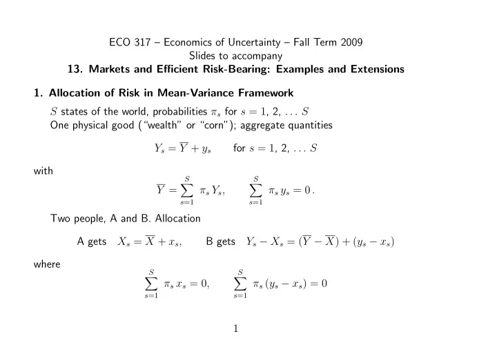
ECO 317 – Economics of Uncertainty – Fall Term 2009 Slides to accompany 13. Markets and Efficient Risk-Bearing: Examples and Extensions 1. Allocation of Risk in Mean-Variance Framework S states of the world, probabilities π s for s = 1 , 2, . . . S One physical good (“wealth” or “corn”); aggregate quantities Y s = Y + y s for s = 1 , 2, . . . S with S S � � Y = π s Y s , π s y s = 0 . s =1 s =1 Two people, A and B. Allocation A gets X s = X + x s , B gets Y s − X s = ( Y − X ) + ( y s − x s ) where S S � � π s x s = 0 , π s ( y s − x s ) = 0 s =1 s =1 1
Mean-variance objectives S S π s ( y s − x s ) 2 . MV A = X − 1 � π s ( x s ) 2 , MV B = ( Y − X ) − 1 � 2 α A 2 α B s =1 s =1 Efficient allocation: choose X , ( x s ) to max MV A subject to MV B ≥ k . Varying k over its range will trace out the Pareto frontier. Lagrangian (with multipliers λ , µ ): S S S � � � � π s ( y s − x s ) 2 − k X − 1 � π s ( x s ) 2 ( Y − X ) − 1 � � L = 2 α A + λ 2 α B + µ π s x s s =1 s =1 s =1 For non-end-point maximization over X , ∂ L ∂X = 1 − λ = 0 . Then S S S π s ( x s ) 2 − 1 π s ( y s − x s ) 2 − k + µ L = Y − 1 � � � 2 α A 2 α B π s x s . s =1 s =1 s =1 So varying k varies X over its range and traces Pareto frontier. 2
With respect to each x σ , ∂ L = − α A π σ x σ + α B π σ ( y σ − x σ ) + µ π σ = 0 ∂x σ Sum over σ and use conditions on sums of deviations and probabilities − α A ∗ 0 + α B ∗ 0 + µ ∗ 1 = 0 or µ = 0 . Then − α A π σ x σ + α B π σ ( y σ − x σ ) = 0 Yielding the solution α B α A x σ = y σ , y σ − x σ = y σ α A + α b α A + α b So each bears risk in inverse proportion to his/her coefficient of risk aversion. When moral hazard is introduced, this will be modified for incentive reasons. 3
2. Incomplete Markets – Example One physical good, corn. There are two farmers, A and B. Each is subject to risk. A: Output,30 or 10, probabilities 1 2 each (mean µ A = 20 , std. dev. σ A = 10 ) B: Output 40 or 0, probabilities 1 2 each (mean µ B = 20 , std. dev. σ B = 20 ) Independent risks. Four states of the world, probabilities 1 4 each. Aggregate outputs (A’s label first) HH: 70; LH : 50; HL: 30; LL : 10 Mean aggregate output Y = 40 , deviations y s = respectively 30, 10, − 10 and − 30 . Mean-variance objective (utility) functions 5 σ 2 20 σ 2 MV A = µ A − 1 MV B = µ B − 1 A B Constant absolute risk aversion coefficients α A = 2 1 5 , α B = 10 . Without any trade in risk, utility levels MV A = 20 − 1 MV B = 20 − 1 5 100 = 0 20 400 = 0 . Think of the zeroes as choice of origin of utility. 4
Pareto Efficient Allocation: A is four times as risk-averse as B, so the deviations should go A: 6 , 2 , − 2 , − 6; B: 24 , 8 , − 8 , − 24 . Resulting variances: A: 20, B: 320. Utilities: MV A = X − 4 , MV B = 40 − X − 16 = 24 − X. So any X in the interval (4,24) is Pareto superior to no trade. Pareto frontier: MV A + MV B = 20 . May have further restrictions to keep quantities non-negative in each state. Allocation Using Shares: B gets fraction φ of A’s farm, A gets fraction (1 − ψ ) of B’s farm. Table of final consumption quantities: State HH LH HL LL A 30(1 − φ ) + 40(1 − ψ ) 10(1 − φ ) + 40(1 − ψ ) 30(1 − φ ) 10(1 − φ ) B 30 φ + 40 ψ 10 φ + 40 ψ 30 φ 10 φ 5
Varying ( φ, ψ ) over a large grid of values in the unit square produces feasible set and frontier using shares to reallocate risk, and comparison with full Pareto efficient frontier. Full efficiency is possible only exceptionally, at (4, 16), with X = 8 . 6
3. Incomplete Markets – Constrained Efficiency? Can have a market where A and B trade shares in their enterprises. Can social planner improve on such a competitive general equilibrium using only shares (not full AD securities) for reallocation purposes? Two people A , B . States s = 1 , 2, . . . S . Endowments ( X 0 i 1 , X 0 i 2 , . . . X 0 iS ) for i = A , B . Final consumption quantities ( X i 1 , X i 2 , . . . X iS ) . Feasible allocation: X As + X Bs ≤ X 0 As + X 0 Bs for all s . Utilities U i ( X i 1 , X i 2 , . . . X iS ) for i = A , B . Ideal full Pareto efficiency for comparison: All the X is are independent choice variables. Usual Pareto efficiency conditions. For any two states s , t : ∂U A /∂X As = ∂U B /∂X Bs ∂U A /∂X As = ∂U A /∂X At , so , ∂U A /∂X At ∂U B /∂X Bt ∂U B /∂X Bs ∂U B /∂X Bt Therefore for all states s , ∂U A /∂X As = θ . ∂U B /∂X Bs 7
Using shares only, reallocations are restricted to two degrees of freedom: X As = (1 − φ ) X 0 As + (1 − ψ ) X 0 X Bs = φ X 0 As + ψ X 0 Bs , Bs . So efficiency condition ∂U A /∂φ ∂U A /∂ψ = ∂U B /∂φ ∂U B /∂ψ or S S S S ∂U A ∂U B ∂U A ∂U A � X 0 � X 0 � X 0 � X 0 As As As Bs ∂X As ∂X Bs ∂X As ∂X As s =1 s =1 s =1 s =1 = , or = = ν S S S S ∂U A ∂U B ∂U B ∂U B � X 0 � X 0 � X 0 � X 0 Bs Bs As Bs ∂X As ∂X Bs ∂X Bs ∂X Bs s =1 s =1 s =1 s =1 Full efficiency implies this condition (with ν = θ ), but not conversely except in very special cases ( S = 2 and output patterns not perfectly correlated). 8
In market, let p = price of A ’s enterprise relative to B ’s. A sells fraction φ of his enterprise to get p φ of B ’s. So X As = (1 − φ ) X 0 As + p φ X 0 Bs . Condition for optimal choice of φ : S ∂U A � X 0 As S ∂X As ∂U A s =1 � [ − X 0 As + p X 0 Bs ] = 0 , or = p . ∂X As S ∂U A s =1 � X 0 Bs ∂X As s =1 Similarly for B . Therefore the constrained efficiency condition is met. However, this result does not generalize to many periods etc. 9
Recommend
More recommend
Explore More Topics
Stay informed with curated content and fresh updates.
