ECO 317 Economics of Uncertainty Fall Term 2009 Slides to - PowerPoint PPT Presentation
ECO 317 Economics of Uncertainty Fall Term 2009 Slides to accompany 19. Price Discrimination by Self-Selection Demand Single consumer: quasilinear utility: u = H ( Q ) + Y , where Q is the quantity (or quality . . . ) of good in question
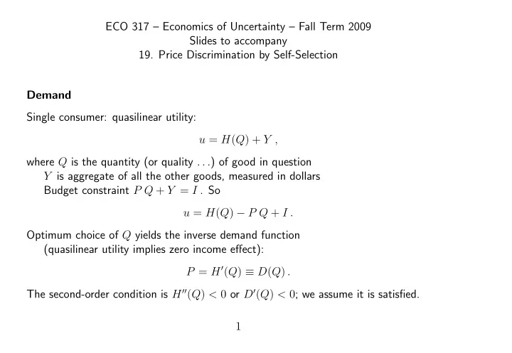
ECO 317 – Economics of Uncertainty – Fall Term 2009 Slides to accompany 19. Price Discrimination by Self-Selection Demand Single consumer: quasilinear utility: u = H ( Q ) + Y , where Q is the quantity (or quality . . . ) of good in question Y is aggregate of all the other goods, measured in dollars Budget constraint P Q + Y = I . So u = H ( Q ) − P Q + I . Optimum choice of Q yields the inverse demand function (quasilinear utility implies zero income effect): P = H ′ ( Q ) ≡ D ( Q ) . The second-order condition is H ′′ ( Q ) < 0 or D ′ ( Q ) < 0 ; we assume it is satisfied. 1
Figure 1 illustrates; demand curve shown straight line purely for convenience. Total utility from this good is area under the curve: � Q H ( Q ) = D ( q ) dq . 0 Revenue is rectangle, consumer surplus is triangle above it. Price H(Q) = whole shaded area Demand curve P = D(Q) Quantity Q Figure 1: Utility and Demand Assume constant marginal cost of production c . 2
Perfect Price Discrimination: One Consumer If monopolist knows D ( Q ) ,can extract full H ( Q ) (all-or-nothing offer or two-part pricing). � Q � Q revenue R ( Q ) = H ( Q ) = D ( q ) dq , profit Π( Q ) = R ( Q ) − c Q = D ( q ) dq − c Q 0 0 Optimum Q = Q ∗ given by Π ′ ( Q ) = D ( Q ) − c = 0 , Price Consumer surplus = Profit Production cost Marginal cost c P = D(Q) Quantity * Q Figure 2: Perfect Price Discrimination with One Consumer 3
Multiple Types; Complete Information Types of consumers labeled i = 1 , 2, . . . n . Population proportions θ i . Inverse demand functions are written D i ( Q ) = H ′ i ( Q ) . ASSUME these are uniformly ranked: D 1 ( Q ) < D 2 ( Q ) < . . . < D n ( Q ) for all Q , or H ′ 1 ( Q ) < H ′ 2 ( Q ) < . . . < H ′ n ( Q ) for all Q . This will be the Mirrlees-Spence single crossing condition: Along an indifference curve of Type i in ( Q, Y ) space, Y = u i − H i ( Q ) Marginal rate of substitution − dY/dQ = H ′ i ( Q ) . So indifference curve of the higher type is steeper: indifference curves of different types cross in only one direction. 4
If the monopolist knows individual consumer’s type (and can use this), can extract all of H i ( Q ) from each type by selling Q ∗ i defined by � Q ∗ i D ′ i ( Q ∗ i ) = c i , and R ∗ i = H i ( Q ∗ i ) = D i ( q ) dq . 0 Economically fully efficient (first-best), but the consumers get no surplus. Figure 3 illustrates this with three types. Price c D 3 D D 1 2 Quantity * * * Q Q Q 3 1 2 Figure 3: Perfect Price Discrimination with Multiple Types of Consumers 5
Incomplete Information – Unavoidable Inefficiency When monopolist does not know individual consumers’ types, or can’t use this. If he tries perfect discrim., consumer can gain by pretending to be lower types. Let u ( i, j ) = utility of a consumer of Type i from offer intended for Type j . u ( i, j ) = H i ( Q ∗ j ) + [ I i − H j ( Q ∗ j ) ] . So H i ( Q ∗ j ) − H j ( Q ∗ u ( i, j ) − u ( i, i ) = j ) � Q ∗ � Q ∗ j j = D i ( q ) dq − D j ( q ) dq 0 0 � Q ∗ j = [ D i ( q ) − D j ( q ) ] dq 0 which is positive when j < i . 6
Figure 4 illustrates this. Price c D 3 D D 1 2 Quantity * * * Q Q Q 1 3 2 Figure 4: Utility Gain From Mimicking Lower Demand Types Shaded area = extra utility of Type 3 pretending to be Type 2. 7
Monopolist’s Optimal Contracts Under Incomplete Information Let ( Q i , R i ) be contract intended for Type i . If Type i buys contract j , u ( i, j ) = H i ( Q j ) − R j + I i . u ( i, i ) − u ( i, j ) = H i ( Q i ) − H i ( Q j ) − R i + R j � Q i � Q j = D i ( q ) dq − D i ( q ) dq − R i + R j 0 0 � Q i = D i ( q ) dq − R i + R j . Q j No imitation (self-selection or incentive-compatibility constraint): � Q i R i ≤ D i ( q ) dq + R j for all j � = i . ( ICall ) Q j And individual rationality or participation constraints � Q i R i ≤ H i ( Q i ) = D i ( q ) dq . ( PC i ) 0 This general formulation allows Q i = Q j and R i = R j ; that is, pooling. Also allows corner solutions Q i = 0 for some i (not serving some type). 8
Steps in analysis: Lemma 1: For any two types j < i , if IC’s hold for this pair, then Q j ≤ Q i . So if all incentive constraints hold, then Q 1 ≤ Q 2 ≤ . . . ≤ Q n . ( Order ) Proof: Choose labels so that j < i . ICs for this pair are � Q i R i − R j ≤ D i ( q ) dq Q j � Q j � Q i R j − R i ≤ D j ( q ) dq = − D j ( q ) dq Q i Q j Adding these together, � Q i 0 ≤ [ D i ( q ) − D j ( q )) ] dq . Q j Since D j ( q ) < D i ( q ) for all q , this implies Q j ≤ Q i . Next, single-crossing property reduces number of ICs from ( n − 1) ∗ n to ( n − 1) . 9
Lemma 2: If (a) the quantities satisfy ( Order ) , and (b) if reduced ICs � Q i R i ≤ D i ( q ) dq + R i − 1 , ( IC i ) Q i − 1 are binding (hold as exact equalities), then all ICs hold. Proof: By example. Consider types 2, 3, 4. � Q 4 � Q 2 u (4 , 4) − u (4 , 2) = D 4 ( q ) dq − D 4 ( q ) dq − R 4 + R 2 0 0 � Q 4 = D 4 ( q ) dq − R 4 + R 2 Q 2 � Q 3 � Q 4 = D 4 ( q ) dq + D 4 ( q ) dq − R 4 + R 2 Q 2 Q 3 � � Q 3 � � Q 4 � � = D 4 ( q ) dq − R 3 + R 2 + D 4 ( q ) dq − R 4 + R 3 Q 2 Q 3 � � Q 3 � � Q 4 � � = D 3 ( q ) dq − R 3 + R 2 + D 4 ( q ) dq − R 4 + R 3 Q 2 Q 3 � Q 3 � Q 3 + D 4 ( q ) dq − D 3 ( q ) dq Q 2 Q 2 10
� Q 3 = [ u (3 , 3) − u (3 , 2) ] + [ u (4 , 4) − u (4 , 3) ] + [ D 4 ( q ) − D 3 ( q ) ] dq . Q 2 So ICs ruling out 3 mimicking 2 and 4 mimicking 3 also rule out 4 mimicking 2. Next consider the possibility that Type 4 wants to mimic Type 5. We have � Q 4 � Q 5 u (4 , 4) − u (4 , 5) = D 4 ( q ) dq − D 4 ( q ) dq − R 4 + R 5 0 0 � Q 4 � Q 5 � � Q 5 � = D 4 ( q ) dq − D 4 ( q ) dq − R 4 + D 5 ( q ) dq + R 4 0 0 Q 4 � Q 5 � Q 5 = − D 4 ( q ) dq + D 5 ( q ) dq Q 4 Q 4 � Q 5 = [ D 5 ( q ) − D 4 ( q ) ] dq , Q 4 Note: going from first to second line assumes that ( IC 5 ) holds as an equality. 11
The monopolist’s profit per capita is n � Π = θ i ( R i − c Q i ) . ( Profit ) i =1 Choose contracts to maximize this subject to: one-step downward ICs ( IC i ) holding as equalities, and PC for the lowest type, ( PC 1 ) . Then verify that all the other PCs for types 2, 3, . . . n also hold. Assume that quantities satisfying ( Order ) ; then by Lemma 2 all ICs hold. So our solution also solution to the full problem. The problem with fewer constraints we solve is called the relaxed problem. At the end, see if the quantities in the solution to the relaxed problem satisfy ( Order ) . 12
Result: for k = 1 2, . . . ( n − 1) , FOC is ∂ Π = θ k [ D k ( Q k ) − c ] − ( θ k +1 + θ k +2 + . . . + θ n ) [ D k +1 ( Q k ) − D k ( Q k ) ] = 0 . ∂Q k Therefore D k ( Q k ) = c + θ k +1 + θ k +2 + . . . + θ n [ D k +1 ( Q k ) − D k ( Q k ) ] > c . θ k So Q k < Q ∗ k : the quantities distorted downward. Purpose: To reduce rent-loss to higher types. For k = n , there are no types h > k . FOC is ∂ Π = θ n [ D n ( Q n ) − c ] = 0 , so D n ( Q n ) = c , ∂Q n no distortion for the best type. Want to keep all the R i as high as possible. So set R 1 at its max: The worst type gets no rent. Others get just enough to meet successive ICs. 13
Price D 5 D 4 D 3 D 2 D 1 c Quantity * * * * Q Q Q Q 2 3 4 1 Q 5 Q Q Q Q 3 4 1 2 Figure 5: Quantities and Payments for Incentive Compatibility 14
Price D 5 D 4 D 3 B D 2 A D 1 c Quantity * * * * Q Q Q Q 2 3 4 1 Q 5 Q Q Q Q 3 4 1 2 Q + 3 Figure 6: Effects of Marginal Changes in Quantities 15
Recommend
More recommend
Explore More Topics
Stay informed with curated content and fresh updates.
