1. Linear Incentive Schemes Denote the agents effort by x and the - PDF document

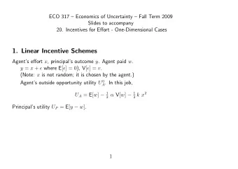
ECO 317 – Economics of Uncertainty – Fall Term 2009 Notes for lectures 20. Incentives for Effort - One-Dimensional Cases Here we consider a class of situations where a principal (such as an owner, or an upper- tier manager, or a downstream user of a product) engages an agent (a manager, or a worker, or an upstream producer of the input in the respective cases). The principal’s outcome depends on the agent’s effort, and also on some other random influence. The effort is the agent’s private information. It is not directly verifiable, and because of the random influence, it cannot be inferred accurately from observing the outcome. Therefore a contract between the two parties that stipulates a payment to the agent conditioned on his effort, although this may be in the ex ante interests of both parties, is not feasible. Exerting effort is costly to the agent; therefore he has an ex post temptation to shirk and blame any bad outcome on bad luck (unfavorable realization of the random component). Thus the situation is one of moral hazard. We consider two models in some detail. These are deliberately abstracted from some aspects of reality, so as to get some basic ideas across in the simplest possible way. In subsequent handouts we will generalize some of these to more realistic situations of multiple tasks, multiple agents, and even multiple principals. We will not go into other issues such as relational contracts without external enforcement. 1. Linear Incentive Schemes Denote the agent’s effort by x and the principal’s outcome by y , and assume y = x + ǫ , (1) where ǫ is a random “observation error” or “noise” with zero expectation (E( ǫ ) = 0) and variance V[ ǫ ] = v . The zero expectation assumption is harmless, as any non-zero expectation can be separated out into the non-random part of the formula for y . Denote the principal’s payment to the agent by w ; this can be a random variable. The agent chooses x to maximize a mean-variance objective function also incorporating a cost of effort: 2 k x 2 . U A = E[ w ] − 1 2 α V[ w ] − 1 (2) Denote the agent’s outside opportunity utility by U 0 A . Therefore the agent’s participation (or individual rationality) constraint is U A ≥ U 0 A The principal is assumed to be risk-neutral. This is often reasonable in the context of employment, where firms are owned by well-diversified shareholder, and even individual owners being richer are likely to be closer to risk-neutrality. But it is easy to generalize the theory to cases where the owner is risk averse and has a mean-variance objective function; I will ask you to do this in the next problem set. Here the principal’s objective function is U P = E[ y − w ] (3) 1

The principal chooses the payment scheme, namely w as a function of the observable and verifiable y , to maximize U P , subject to the agent’s participation constraint, and the knowledge that the agent is going to choose x to maximize U A , that is, the incentive com- patibility constraint. We begin by laying down a benchmark against which to compare that outcome, namely the situation without asymmetry where the effort can be directly observed and verified, and therefore a Pareto efficient or first-best contract can be implemented. Hypothetical Ideal or First-Best Here the principal can choose a contract of the form ( x, w ), whereby the agent promises to make effort x and the principal promises to pay the agent w , which may be a random variable. The principal will choose these to maximize U P = E[ y − w ] = E[ x + ǫ − w ] = x − E[ w ] , subject only to the agent’s participation constraint 2 k x 2 ≥ U 0 U A = E[ w ] − 1 2 α V[ w ] − 1 A . Obviously the principal will not give the agent any more than he has to, so the participation constraint holds with equality. We can then substitute out E[ w ] in U P to write 2 k x 2 − U 0 U P = x − 1 2 α V[ w ] − 1 A . The value of x that maximizes this satisfies the first-order condition 1 − 1 2 2 k x = 0 , therefore x = 1 /k . (4) (The second-order condition is − 2 k ≤ 0, which is true.) As for w , its choice should minimize V[ w ], so w should be non-random. This is intuitive: since the principal is risk-neutral, it is efficient for him to bear all the risk, and since effort is directly verifiable (information is complete), there are no incentive reasons to make the agent bear any risk either. Then, using the participation constraint, we have A + 1 2 k x 2 = U 0 w = U 0 A + 1 2 k , using the optimized value of x . Finally, the two parties’ overall utility levels are U A = U 0 A , and U P = 1 2 k − U 0 (5) A The agent is on his participation constraint and gets no surplus. The principal gets all the surplus that exists in the relationship. Of course it is possible that U 0 A < 1 / (2 k ). In that case it would be optimal not to enter into this contract, and let the agent take up the outside opportunity. (The principal’s outside opportunity has been implicitly assumed to be zero.) 2

Second-Best Linear Incentive Schedules Now the payment w to the agent must be conditioned on the only verifiable magnitude in the interaction, namely y . In fact we will consider a simple special case where w has to be a linear (affine, if you want to be pedantic) function of y , say w = h + s y . (6) Here h is the basic wage and s is a performance-based bonus coefficient. So the principal’s problem is reduced from one of choosing a whole function w ( y ) optimally to that of choosing just the two parameters h and s optimally. In later sections we will examine some simple ideas about nonlinear payment schemes. We have w = h + s ( x + ǫ ) = ( h + s x ) + s ǫ , rearranging to separate out the non-random and random terms. Therefore V[ w ] = s 2 V[ ǫ ] = s 2 v , E[ w ] = h + s x , Then the agent chooses x to maximize 2 α v s 2 − 1 2 k x 2 . U A = h + s x − 1 This has the first-order condition s − 1 2 2 k x = 0 , therefore x = s/k . (7) (The second-order condition is − 2 k ≤ 0, which is true.) Contrast this with the first-best effort level in ( ?? ). The effort level chosen by the agent here is only a fraction s of the first- best, reflecting the fact that the agent receives only the fraction s of the expected marginal product of his effort. For this reason, we will call the coefficient s the power of incentive in this scheme. We will soon obtain the principal’s optimal choice of s , and later contrast it with similar expressions for the power of incentives in other situations. Substituting for the agent’s choice of x into his objective function, we get his maximized or “indirect utility” function: = h + s 2 A = h + s s � s � 2 2 α v s 2 − 1 2 α v s 2 . k − 1 2 k − 1 U ∗ 2 k k The principal’s utility is then U P = E[ y − h − s y ] = (1 − s ) x − h = (1 − s ) s k − h . The principal chooses h and s to maximize this, subject to the agent’s incentive compatibility and participation constraints. The former is simply ( ?? ), and has already been incorporated A ≥ U 0 into the agent’s utility expression. There remains only the participation constraint U ∗ A , or h + s 2 2 α v s 2 ≥ U 0 2 k − 1 A . 3

It is obviously not optimal for the principal to leave any slack in this constraint. Therefore we can replace the ≥ by = and use this equation to substitute out for h in the principal’s objective: A − s 2 2 α v s 2 . h = U 0 2 k + 1 (8) Therefore + s 2 s (1 − s ) 2 α v s 2 − U 0 2 k − 1 U P = A k k − s 2 s 2 α v s 2 − U 0 2 k − 1 = A . The only remaining choice variable is s . The first-order condition is k − s 1 k − 1 2 α v (2 s ) = 0 ; the second-order condition is obviously met. Solving the first-order condition, therefore the optimum is 1 s = 1 + α v k . (9) This formula yields some very nice and simple intuitive interpretations: [1] In general, 0 < s < 1. We saw in the first-best that if it were not for the information asymmetry, it would be efficient for the risk-neutral principal to absorb all the risk, leaving the agent with a non-random income. Then s would equal zero. On the other hand, if there is information asymmetry, the only way to induce the agent to exert a level of effort equal to the first best (1 /k ) is to have s = 1, thereby giving the agent the full marginal expected return to his effort. (The total payment to the agent can be adjusted by choosing the fixed component of the payment, namely h , appropriately.) In general, the optimal s strikes a balance between the risk-bearing and the incentive purposes. [2] The higher is α , the lower is s . The intuition is as follows. A high s makes the agent’s income more random (risky). The principal must then offer the agent a higher fixed payment h to continue fulfilling the participation constraint. This gets more and more costly ( h increases with s 2 ), and the effect is more pronounced when α is higher, as ( ?? ) shows. Therefore a higher α entails a lower s . [3] The higher is v , the lower is s . A high v means that the error or noise term ǫ in the outcome y is likely to be bigger. Then paying the agent for a higher y may too often be rewarding him for good luck, or punishing him for bad luck. The agent does not like this risk, and again the principal must raise the fixed payment to meet the participation constraint. It is better for the principal to lower the s to some extent. [4] Substituting the formula ( ?? ) back into the principal’s objective, we find its maximized value: 1 2 k (1 + α v k ) − U 0 U P = A . (10) Comparing this with the corresponding expression ( ?? ) in the full information, first best case, we see the loss caused by the information asymmetry. The principal bears this loss; 4