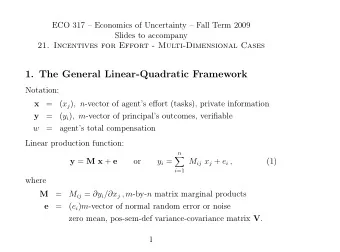
1. The General Linear-Quadratic Framework Notation: x = ( x j ) , - - PDF document

ECO 317 – Economics of Uncertainty – Fall Term 2009 Notes for lectures

• 21. Incentives for Effort - Multi-Dimensional Cases

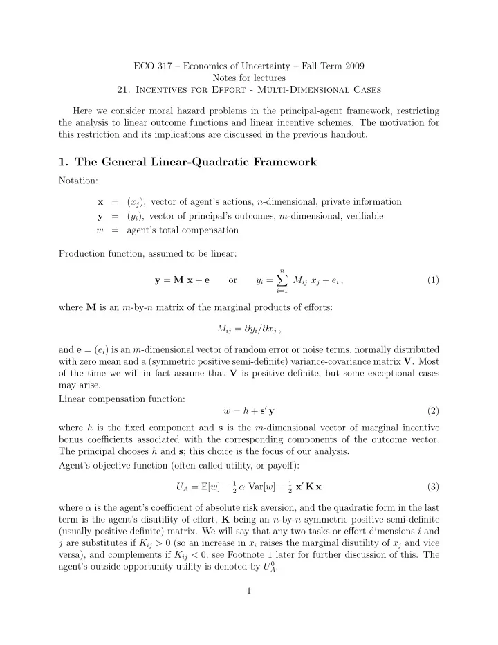
Here we consider moral hazard problems in the principal-agent framework, restricting the analysis to linear outcome functions and linear incentive schemes. The motivation for this restriction and its implications are discussed in the previous handout.

• 1. The General Linear-Quadratic Framework

Notation: x = (xj), vector of agent’s actions, n-dimensional, private information y = (yi), vector of principal’s outcomes, m-dimensional, verifiable w = agent’s total compensation Production function, assumed to be linear: y = M x + e

• r

yi =

n

• i=1

Mij xj + ei , (1) where M is an m-by-n matrix of the marginal products of efforts: Mij = ∂yi/∂xj , and e = (ei) is an m-dimensional vector of random error or noise terms, normally distributed with zero mean and a (symmetric positive semi-definite) variance-covariance matrix V. Most

• f the time we will in fact assume that V is positive definite, but some exceptional cases

may arise. Linear compensation function: w = h + s′ y (2) where h is the fixed component and s is the m-dimensional vector of marginal incentive bonus coefficients associated with the corresponding components of the outcome vector. The principal chooses h and s; this choice is the focus of our analysis. Agent’s objective function (often called utility, or payoff): UA = E[w] − 1

2 α Var[w] − 1 2 x′ K x

(3) where α is the agent’s coefficient of absolute risk aversion, and the quadratic form in the last term is the agent’s disutility of effort, K being an n-by-n symmetric positive semi-definite (usually positive definite) matrix. We will say that any two tasks or effort dimensions i and j are substitutes if Kij > 0 (so an increase in xi raises the marginal disutility of xj and vice versa), and complements if Kij < 0; see Footnote 1 later for further discussion of this. The agent’s outside opportunity utility is denoted by U 0

A.

1

Principal’s objective function (often called utility, or payoff): UP = E[p′ y − w] (4) where p is the vector of valuations the principal places on the corresponding compnents of the outcome vector. Thus the principal is assumed to be risk-neutral. The theory is easy to extend to the case where the principal also has a mean-variance objective function.

• 2. One Principal, One Agent

We have w = h + s′ y = h + s′ M x + s′ e Therefore E[w] = h + s′ M x , Var[w] = s′ V s and UA = h + s′ M x − 1

2 α s′ V s − 1 2 x′ K x

(5) The agent chooses x to maximize this. The first-order condition is M′ s − K x = 0 . (6) The second-order condition is that the matrix − K is negative semi-definite, which is true because K is positive semi-definite. If you can do differentiation with respect to vector arguments directly, this is all you need to say. Otherwise you can verify the result by writing

• ut the vector and matrix products in full. I will do this once in this instance, and leave

similar future calculations to you. The objective function written out in full is UA = h +

m

• i=1

n

• j=1

si Mij xj − 1

2 m

• i=1

m

• k=1

si Vik sk − 1

2 n

• h=1

n

• j=1

xh Khj xj . For any one component of x, say xg, we have ∂UA ∂xg =

m

• i=1

si Mig − 1

2 n

• h=1

xh Khg − 1

2 n

• j=1

Kgj xj . Rearranging and collecting terms into vector and matrices yields (6). In the process, the matrices M and K have to be transposed, and you need to remember that the latter is symmetric. Solving the first-order condition (6) for x yields the agent’s effort choice: x = K−1 M′ s . (7) As usual, this becomes the incentive compatibility condition on the principal’s choice. Substituting this into the production function (1) and taking expectations, we have E[y] = M K−1 M′ s ≡ N s , 2

where I have defined the symmetric and positive semi-definite matrix N = M K−1 M′ . (8) This elements of this matrix are the marginal products for the principal’s outcomes of the various bonus coefficients: Nij = ∂E[yi]/∂sj , given that the agent chooses his effort response in his own optimal interests. Substituting from the incentive compatibility constraint (7) into the expression (5) for the agent’s utility, we get the agent’s maximized or indirect utility function: U ∗

A

= h + s′ M [ K−1 M′ s] − 1

2 α s′ V s − 1 2 [ K−1 M′ s]′ K [ K−1 M′ s]

= h + 1

2 s′ M K−1 M′ s − 1 2 α s′ V s

= h + 1

2 s′ N s − 1 2 α s′ V s

(9) And the principal’s indirect utility function, after substituting the agent’s response, is UP = p′ E[y] − E[w] = p′ N s − h − s′ M [ K−1 M′ s ] = p′ N s − h − s′ N s . (10) The agent’s participation constraint becomes U ∗

A ≥ U 0

• A. This will be binding, so we can

use it as an equation to solve for h and substitute into the principal’s indirect utility function, to make it a function of s alone. This yields UP = p′ N s − U 0

A + 1 2 s′ N s − 1 2 α s′ V s − s′ N s

= p′ N s − U 0

A − 1 2 s′ N s − 1 2 α s′ V s

(11) The first-order condition for s to maximize this is N p − [ N + α V ] s = 0 . (12) Useful exercise to improve your skill in doing such calculations: Verify this by writing out all the matrix products in (11) explicitly and taking the derivatives with respect to the components of s, and then reassemble the result into vector and matrix notation, as was done for (6) above. (The second-order condition is that the matrix (N + α V) should be positive semi-definite, which is true.) Therefore the principal’s optimal choice of the marginal bonus coefficient vector is given by s = [ N + α V ]−1 N p . (13) We can verify that the one-dimensional result(equation (9) in Handout 20) is a special case of this: Take p = 1, M = 1, K = k, and V = v. Then N = 1/k, and (13) becomes s = [(1/k) + α v ]−1 (1/k) = 1 1 + α v k . Thus reassured, we can examine several applications. Although we can do this using the general formula, the intuition for the various issues is better developed by focusing on just

• ne new issue at a time, and simplifying everything else as much as possible.

3

• 3. One Task, Two Outcome Measures

Here we examine the relative merits of different outcome measures. For this purpose, let us take m = 2 and n = 1. Let the matrix M (which is now just a 2-by-1 column vector) with both elements equal to 1; this is just a choice of units. Let the matrix V be diagonal, V =

• v1

v2

• ;

then N =

• 1

1

1

k

• 1

1

• = 1

k

• 1

1 1 1

• ,

and N + α V = 1 k

• 1 + k α v1

1 1 1 + k α v2

• .

Therefore s = k

• 1 + k α v1

1 1 1 + k α v2

−1 1

k

• 1

1 1 1

• p ,
• r
• s1

s2

• =

1 1 + k α v1 + k α v2 + k2 α2 v1 v2 − 1

• 1 + k α v2

−1 −1 1 + k α v1 1 1 1 1 p1 p2

• .

This simplifies to s1 = v2 (p1 + p2) v1 + v2 + k α v1 v2 , s2 = v1 (p1 + p2) v1 + v2 + k α v1 v2 . This yields the following results:; [1] Suppose output 2 is worth less to the principal; p2 could even be zero. Even then, we have s2 = 0. In fact, each of s1 and s2 depends only on the sum (p1 + p2), which is the expected contribution to the principal’s value (coming from both outcomes) of an extra unit

• f the agent’s effort. Outcome 2 will remain useful even when its direct value to the principal

equals zero, because it furnishes additional verifiable information about the agent’s effort. In fact, the ratio s1/s2 is just v2/v1, inverse of the ratio of the variances of the error or noise terms in the two outcomes, and nothing else. If v1 is large compared to v2, then s2 will be large compared to s1. If outcome 2 is much more informative than outcome 1, then it may be used exclusively. In the limit, if p2 = 0 and v1 → ∞, we have s1 → 0, s2 → p1 1 + k α v2 . [2] The agent’s risk aversion is no longer crucial. Even if α = 0, each of s1 and s2 is < (p1 + p2). Specifically, s1 = v2 (p1 + p2) v1 + v2 , s2 = v1 (p1 + p2) v1 + v2 . Thus s1 +s2 = p1 +p2, so the sum of the bonus coefficients does equal the sum of principal’s valuations of the two components of the outcomes resulting from a unit increase in the agent’s

• effort. Thus, with a risk-neutral agent and two outcome measures, the total incentive has

full power, but its split between the two outcome measures is optimally designed to achieve greater informativeness. 4

• 4. Many tasks, Two Outcomes

The dimension n of the agent’s action vector x is often quite large. Suppose the outcome vector is two-dimensional. The principal values only dimension 1, so p2 = 0. But outcome 1 is unverifiable, so the principal is constrained to set s1 = 0. Let us also take α = 0 to remove the issue of the agent’s risk aversion, as it is not essential in this context. Similarly, assume K is diagonal with entries k each, that is K = k In where In is the n-by-n identity matrix, in order to remove issues of complementarity or substitution among the agent’s actions, and also of any differences in disutilties across the dimensions of effort. With all this, UP = ( p1 0 )

• N11

N12 N21 N22 s2

• − 1

2 ( 0 s2 )

• N11

N12 N21 N22 s2

• =

p1 N12 (s2)2 − 1

2 N22 (s2)2 .

The first-order condition (12) for s2 (the only relevant component of s) becomes N22 s2 = N12 p1 . Also N = M (k In)−1 M′ = 1 k M M′ . Therefore N22 = 1 k

n

• j=1

(M2j)2 , N12 = 1 k

n

• j=1

M1j M2j , and then s2 =

n

• j=1

M1j M2j

n

• j=1

(M2j)2 p1 . The sign of s2 is the same as the sign of the sum in the numerator on the right hand side, and the magnitude of s2 also depends importantly on the magnitude of that numerator. The interpretation or intuition is as follows. The numerator shows how well or poorly aligned across the many dimensions of the agent’s actions are the marginal effects of the actions on the two dimensions of outcome, the first which matters directly to the principal but is unverifiable, and the second which has no direct value to the principal but is the

• nly verifiable indicator on which the payments to the agent can be based. The available

indicator is good if it is well aligned in this sense with what the principal values. A large negative alignment would be just as valuable as a large positive alignment. If N21 is negative, then principal need only make s2 negative, that is, penalize the agent if the indicator y2 is

• high. The fixed component h can adjust to ensure fulfillment of the agent’s participation
• constraint. What would make the indicator useless is a zero alignment, namely the two

vectors (M1j) and (M2j) being orthogonal to each other in n-dimensional space. 5

• 5. Substitutes and Complements in Efforts

Now focus on the situation where the different dimensions of the agent’s effort are not additively separable in disutility, that is, the matrix K has non-zero off-diagonal entries. Again get rid of all the other, now inessential, features: suppose that [1] there are just two dimensions of actions and outcomes, [2] the principal values the two outputs equally, with p1 = p2 = p, [3] the production function matrix M is diagonal, in fact the identity matrix I2, so action 1 affects only outcome 1 and action 2 affects only outcome 2, with expected marginal products normalized to 1 in each case, [4] the error variance matrix V is also diagonal and equal to v I2, so there is no difference in the informativeness of the two

• utcome measures, and [5] the disutility matrix is

K =

• k

θ k θ k k

• .

where k > 0 and −1 < θ < 1. So the actions are substitutes if θ > 0 and complements if θ < 0. To see the substitutes versus complements issue in a different light, consider what happens to the agent’s effort choices given by (7). With all the special assumptions now made, we get x = K−1 I2 s = K−1 s , so

• x1

x2

• =
• k

θ k θ k k

−1

s1 s2

• =

1 k

• 1

θ θ 1

−1

s1 s2

• =

1 k (1 − θ2)

• 1

− θ − θ 1 s1 s2

• =

1 k (1 − θ2)

• s1 − θ s2

s2 − θ s1

• (14)

Therefore when efforts are substitutes (θ > 0), increasing the bonus coefficient on one task increases the effort the agent devotes to that task, at the expense of the effort devoted to the other task. When efforts are complements (θ < 0, an increase in either s1 or s2 increases both x1 and x2.1 This in turn affects the principal’s choice of the incentive bonus coefficients. To see this, begin by observing that with our simplifying assumptions, N = I2 K−1 I2 = K−1 ,

1Alas, this alternative way of viewing substitution and complementarity are no longer equivalent when

n ≥ 3. This is analogous to the difference between the Allen and the Hicks definitions of substitutes and complements in standard demand theory. If you don’t know that material from ECO 310, just keep this footnote stored somewhere in your mind just in case it becomes necessary when you are reading more advanced literature on the subject.

6

so the first-order condition (12) becomes [ K−1 + α v I2 ] s = K−1 p . Premultiplying by K gives [ I2 + α v K ] s = p ,

• r
• 1 + α v k

θ α v k θ α v k 1 + α v k s1 s2

• =
• p

p

• .

This yields the solution s1 = s2 = p 1 + (1 + θ) α v k . Thus, when θ > 0, that is, the two tasks are substitutes in the agent’s utility, the interaction makes it necessary for the principal to reduce the power of incentives on both

• utcomes, because sharpening the incentives on either will cause the agent to divert his

effort away from the other, as the agent’s choice equation (14) shows. Conversely, if θ < 0 (complements), then a stronger incentive to one task causes the agent to increase the effort

• n both, so more powerful incentives on both tasks become optimal for the principal.

This has implications for the next level of analysis, namely organization theory. If you need multiple tasks performed, and have a choice of grouping them for assignment to different agents (or agencies or bureaucracies), then you should group them in such a way that each agent is assigned a set of mutually complementary tasks, not mutually substitute ones. Think of some organizations you know – universities, the IRS, Homeland Security – and think whether they follow this principal, and if not, with what results.

• 6. Multiple Principals – Common Agency (Optional)

In many situations, one person takes some privately observable actions that have multidi- mensional verifiable outcomes. Several people care differently about the different outcomes, and have the ability to reward (or punish) the person responsible for the actions based on the

• utcomes. This situation is referred to as a common agency. The person taking the actions

is the common agent of all the principals who care about the outcomes. Two examples: [1] politicians and bureaucratic agencies of the government are common agents to a set of principals that includes the public, the judiciary, the media, . . . [2] professors share research assistants and secretaries. In such situations, the payoffs and compensation may be non- monetary in part, for example special interests may campaign or vote against a politician who fails to deliver the outcomes they want, and a professor can vary the quality of letters

• r recommendation for a former research assistant!

The notation stated at the beginning of the handout continues. Once again I keep things as simple as possible by ignoring all inessential complications. So suppose there are two actions and two outcomes (m = n = 2). The production function matrix M is the 2- by-2 identity matrix I2; so action 1 contributes only to outcome 1 and action 2 only to 7

• utcome 2. The disutility of effort is separable, so K = k I2 and there is no substitution or

complementarity between the tasks. Then N = I2 1 k I2 I2 = 1 k I2 The error variance matrix is also diagonal and symmetric between the tasks, V = v I2. If the two principals got together and jointly decided on the incentive scheme, we would find s1 = p1 1 + α v k, s2 = p2 1 + α v k (15) The main purpose of this analysis is to compare this jointly optimal decision with the Nash equilibrium of the game between the principals when they act independently, that is, find the cost to the principals of failing to act cooperatively. So now let the two principals act independently. Write their total compensation schedules w1 = h1 + s1,1 y1 + s1,2 y2 (16) w2 = h2 + s2,1 y1 + s2,2 y2 (17) In the notation for the bonus coefficients, the first subscript refers to the principal and the second to the outcome; thus s2,1 is the bonus coefficient set by principal 2 on outcome 1. Note that both principals are setting bonus coefficients on both dimensions of outcome even though each is directly concerned with only one dimension. The purpose is of course to affect the agent’s action in a way that benefits oneself; we examine the implications of this. We have a game of strategy between the principals. The strategy of principal 1 is the triple (h1, s1,1, s1,2) and that of principal 2 is the triple (h2, s2,1, s2,2). We seek the Nash equilibrium

• f their game. For this, they must calculate the payoffs (expected utilities) resulting from

their strategy choices, and in doing so, they must take into account the common agent’s responses. The total compensation package for the agent, obtained by summing the two principals’ schedules, is w = h + s1 y1 + s2 y2 where h = h1 + h2, s1 = s1,1 + s2,1, s2 = s1,2 + s2,2 Then, from (7) the agent’s effort choice is given by

• x1

x2

• =
• 1/k

1/k 1 1 s1 s2

• r x = s / k or

x1 = s1 k = s1,1 + s2,1 k , x2 = s2 k = s1,2 + s2,2 k 8

Then E[w1] = h1 + s1,1 x1 + s1,2 x2 = h1 + s1,1 s1 k + s1,2 s2 k = h1 + 1 k [ s1,1 (s1,1 + s2,1) + s1,2 (s1,2 + s2,2) ] Next, substituting the special forms of N and V appropriate to the present context into the agent’s indirect utility function expression (9), we have U ∗

A

= h + 1 2k s′ s − 1 2 α v s′ s = h1 + h2 +

1

2k − α v 2 (s1,1 + s2,1)2 + (s1,2 + s2,2)2 (18) Now consider one of the principals, say principal 1. His utility is U 1

P = E[ p1 y1 − w1 ] = p1

s1,1 + s2,1 k − h1 − 1 k [ s1,1 (s1,1 + s2,1) + s1,2 (s1,2 + s2,2) ] He wants to maximize this, given principal 2’s strategy (h2, s2,1, s2,2) and respecting the agent’s participation constraint U ∗

A ≥ U 0

• A. From (18) we see that to meet the constraint,

principal 1 must set h1 = U 0

A − h2 −

1

2k − α v 2 (s1,1 + s2,1)2 + (s1,2 + s2,2)2 Substituting this in principal 1’s utility function, we have U 1

P

= p1 s1,1 + s2,1 k − U 0

A + h2 +

1

2k − α v 2 (s1,1 + s2,1)2 + (s1,2 + s2,2)2 −1 k [ s1,1 (s1,1 + s2,1) + s1,2 (s1,2 + s2,2) ] To maximize this with respect to s1,1 and s1,2, the first-order conditions are 1 k p1 +

1

2k − α v 2

• 2 (s1,1 + s2,1) − 1

k (2 s1,1 + s2,1) =

1

2k − α v 2

• 2 (s1,2 + s2,2) − 1

k (2 s1,2 + s2,2) =

• r

p1 − (1 + α v k) s1,1 − α v k s2,1 = −(1 + α v k) s1,2 − α v k s2,2 = These can be solved for principal 1’s strategies (s1,1, s1,2) in terms of principal 2’s strategies (s2,1, s2,2); those solutions will constitute principal 1’s “best response” or “reaction func- tions”. 9

Similarly, for principal 2, we get the conditions p2 − (1 + α v k) s2,2 − α v k s1,2 = −(1 + α v k) s2,1 − α v k s1,1 = defining his best response or reaction functions. Solving all four together will yield the Nash equilibrium values of the strategies (s1,1, s1,2) and (s2,1, s2,2). The first equation in principal 1’s conditions and the second equation in principal 2’s conditions involve only s1,1 and s2,1; therefore those equations can be solved for these two

• unknowns. The result is

s1,1 = 1 + α v k 1 + 2 α v k p1, s2,1 = − α v k 1 + 2 α v k p1 These are the bonus incentives offered by the two principals for outcomes with regard to the first dimension of outcome. Then the aggregate bonus coefficient for the first dimension

• f outcome is

s1 = s1,1 + s2,1 = 1 1 + 2 α v k p1 The separate principals’ choices and the aggregate bonus coefficient for the second dimension can be solved symmetrically. The solutions reveal how each principal reacts to the presence of the other and the task that benefits the other. Each offers a positive bonus coefficient for the dimension that benefits himself, and in fact it can be seen that this coeffcient is stronger than that offered under joint maximization, that is 1 + α v k 1 + 2 α v k > 1 1 + α v k But each principal offers a negative bonus coefficient on the dimension of the outcome that benefits the other principal! For principal 1, for example, this is a relatively less costly way to reduce the agent’s effort and therefore the agent’s disutility, thereby being able to reduce the fixed salary component while meeting the participation constraint. This aspect (negative incentives on the other dimension) would be exacerbated if the tasks were substitutes in the agent’s disutility. When both principals are behaving in this way, the aggregate incentives for the agent become weaker; the sum of the bonus coefficients coming from the two principals in the Nash equilibrium is less than that in formula (15) where the principals act jointly: 1 1 + 2 α v k < 1 1 + α v k If there are n principals, the 2 in the denominator is replaced by n; so the incentives weaken dramatically as the number of principals increases. If each principal could not observe the other’s outcome, or was forbidden from condi- tioning his incentives on the other’s outcome, the power of incentives could be restored even 10

with independent action. Thus, if s2,1 is constrained to equal 0, then principal 1’s first order condition with respect to s1,1 becomes p1 − (1 + α v k) s1,1 = 0

• r

s1 = s1,1 = 1 1 + α v k p1 as in the joint optimum (15); similarly for the other principal. However, in reality, and especially in political contexts, it is difficult to compartmentalize information or to restrict the principals’ choice of incentive schedules for their common agent.

• 7. Multiple Agents – Relative Performance Schemes (Optional)

If one principal oversees several agents performing similar tasks, then schemes that compen- sate each based on his performance relative to that of the others are sometimes used. Here we find the incentive rationale for these. As usual, we simplify the inessential aspects of the problem. So we consider one principal

• verseeing two agents, each of whom contributes to the principal’s outcome independently,

but with correlated errors. Thus y1 = x1 + e1, y2 = x2 + e2 where (e1, e2) are jointly normal with mean (0, 0) and variance-covariance matrix V =

• v

ρ v ρ v v

• We also let the principal’s valuations of the outputs p1 = p2 = 1.

Write the compensation schedule for agent 1 as w1 = h1 + s1,1 y1 + s1,2 y2 In the bonus coefficients, the first subscript indicates the agent and the second the outcome. Note that the agent’s compensation depends in part on the outcome y2 which he does not control at all; we will see the reason for this soon. Usual calculations show that E[w1] = h1 + s1,1 x1 + s1,2 x2 and Var[w1] = ( s1,1 s1,2 ) V

• s1,1

s1,2

• =

v (s1,1)2 + 2 ρ v s1,1 s1,2 + v (s1,2)2 11

The agent chooses x1 to maximize U 1

A

= E[w1] − 1

2 α Var[w1] − 1 2 k (x1)2

= h1 + s1,1 x1 + s1,2 x2 − 1

2 α Var[w1] − 1 2 k(x1)2

This yields the first order condition s1,1 − k x1 = 0 so x1 = s1,1 / k Similarly for agent 2, x2 = s2,2 / k in analogous notation. Substituting these, agent 1’s maximized or indirect utility function is U ∗1

A = h1 + (s1,1)2

k + s1,2 s2,2 k − 1

2 α Var[w1] − (s1,1)2

2k A similar expression can be found for agent 2’s indirect utility function. The principal’s payoff is UP = E[y1 + y2 − w1 − w2] = x1 + x2 − E[w1] − E[w2] As usual, we (1) substitute the agents’ choices of the xi as functions of the respective bonus coefficients (incorporate the incentive constraints), and (2) use the participation constraints U ∗i

A ≥ U 0i A (where the outside opportunities U 0i A are exogenously given) to solve out for the

constant terms h1 and h2 in the compensation schedules. Then, the principal’s objective becomes a function of the bonus coefficients alone: UP = s1,1 k − U 01

A − 1 2 α Var[w1] − (s1,1)2

2k +s2,2 k − U 02

A − 1 2 α Var[w2] − (s2,2)2

2k For notational convenience, I have not written out the full expressions for the variances. It remains to maximize this with respect to the four bonus coefficients. For those per- taining to agent 1, we have the first order conditions ∂UP ∂s1,1 = 1 k − 1

2 α [ 2 v s1,1 + 2 v ρ s1,2 ] − s1,1

k = 0 ∂UP ∂s1,2 = −1

2 α [ 2 v ρ s1,1 + 2 v s1,2 ] = 0

• r

[ 1 + k v α ] s1,1 + ρ k v α s1,2 = 1 and s1,2 = −ρ s1,1 12

These yield s1,1 = 1 1 + k v α (1 − ρ2), s1,2 = − ρ 1 + k v α (1 − ρ2) The effect is better seen by writing out the full schedule: w1 = h1 + y1 − ρ y2 1 + k v α (1 − ρ2) Thus as usual agent 1 is rewarded if his outcome is higher, but now, if ρ is positive, he is penalized if the other agent’s output is higher. In fact, if the correlation is perfect, so ρ = 1, then w1 = h1 + (y1 − y2) so the incentive (non-constant) part of the compensation depends purely on the relative

• utcomes. The intuition is this.

y1 − y2 = (x1 − x2) + (e1 − e2) and Var(e1 − e2) = Var(e1) + Var(e2) − 2 ρ [Var(e1) Var(e2)]1/2 = 2 v (1 − ρ) which is zero if ρ = 1. Therefore in that case, (y1 − y2) gives the principal perfect infor- mation about (x1 − x2), and with the agents acting independently, this amounts to perfect information about x1 and x2 separately. Of course this compensation scheme is vulnerable to collusion between the agents. Other issues arising when one principal has several agents: The principal’s total outcome may not be additively separable across the agents’ actions, but instead a production function y = F(x1, x2, . . .) with complementarity. This is a problem of “moral hazard in teams”.

Readings

The material of Sections 1–5, and some of 7, is basically an exposition of the Holmstrom- Milgrom “Multitask Principal-Agent Analysis” paper on the reading list. Section 6 relies on my “Incentives and Organizations in the Public Sector” paper that is an optional reading and the AER Papers and Proceedings 1997 paper cited there. You don’t have to read those; it is enough to read this handout section. You should read the Gibbons and Prendergast papers

• n the reading list to get an idea of the scope of validity, and various applications, of the

theoretical framework we have begun to develop here. The Holmstr¨

• m and Baron-Myerson

papers on the reading list, while required, are technically difficult, so read them quickly to get a general idea of what they are saying, without going into details of the algebra and calculus. 13