Equilibrium, Welfare & Information ECON 4240, Spring 2018 - PowerPoint PPT Presentation
Equilibrium, Welfare & Information ECON 4240, Spring 2018 Piacquadio & Traeger University of Oslo Piacquadio & Traeger: Equilibrium, Welfare, & Information. UiO Spring 2018. 1/27 Content Part I: Christian Traeger PART I:
Equilibrium, Welfare & Information ECON 4240, Spring 2018 Piacquadio & Traeger University of Oslo Piacquadio & Traeger: Equilibrium, Welfare, & Information. UiO Spring 2018. 1/27
Content Part I: Christian Traeger PART I: Equilibrium & Welfare 1. Partial Equilibrium ◮ Focus on one market ◮ E.g. how tax affects a market 2. General Equilibrium ◮ Feedback between different markets ◮ Welfare theorems on how the markets “perform” 3. Imperfect Competition ◮ How do firms really compete in many markets ◮ E.g. Bertrand/Cournot have very different implications 4. Externalities & Public Goods ◮ Market Failures & Policy fixes ◮ E.g. Pigovian Taxation, Voting Piacquadio & Traeger: Equilibrium, Welfare, & Information. UiO Spring 2018. 2/27
Content Part II: Paolo Piacquadio PART II: Welfare & Information 1. Introduction to asymmetric information ◮ a simple approach ◮ the contract theoretic approach 2. Adverse Selection ◮ example 1: the market for lemons (Akerlof, 1970) ◮ example 2: life insurance (health conditions) 3. Moral Hazard ◮ example 1: a university hiring a researcher ◮ example 2: life insurance (health behavior) Piacquadio & Traeger: Equilibrium, Welfare, & Information. UiO Spring 2018. 3/27
Organizational Items Lecture Schedule: online here General: Thursdays 10:15-12:00 in Auditorium 5 Exceptions: Monday 14:15-16:00 in Auditorium 1 on Feb 5, March 19, Apr 9 [maybe also moving March 8] Seminar Instructor: Vegard Wiborg Seminar Timing: 2 options, Wednesday or Thursday, schedule Term Paper 1 st attempt: out: March 15 in: March 19 Term Paper 2 nd attempt: out: April 3 in: April 6 Exam: May 11 at 9:00 AM (3 hours) in Sal 4D Silurveien 2 Traeger’s office hours (room 1111): Thursdays 1-2pm (1 st half of lecture) or by appointment Prerequisite: Econ 3200/4200 and 3120/4120 (Math 2) Disclaimer: check online for updates Piacquadio & Traeger: Equilibrium, Welfare, & Information. UiO Spring 2018. 4/27
The Partial Equilibrium Competitive Model Lecture 1, ECON 4240 Spring 2018 Snyder et al. (2015) chapter 11 University of Oslo 18.01.2018 Piacquadio & Traeger: Equilibrium, Welfare, & Information. UiO Spring 2018. 5/27
Outline Focus: ◮ Determine the market price of one good, taking price of other goods as given ◮ What’s the use of such a model? ◮ To study the effect of taxes and price regulations ◮ To study the effect of changes in income levels on market prices and quantity of goods sold ◮ To think about how the gains from trade are divided between sellers and buyers (guide redistribution policy?) ◮ To have a benchmark for later studying potential welfare losses from the lack of competition (oligopolies) ◮ ... and much more... Piacquadio & Traeger: Equilibrium, Welfare, & Information. UiO Spring 2018. 6/27
The Market Demand Curve I ◮ ECON 4200 (see Part 2 of Snyder et al. (2015)): Let there be two goods available (good x and good y ). The individual demand function for good x x i ( p x , p y , I i ) characterizes the quantity demanded of good x by consumer i as a function of market prices p x , p y and consumer i ’s monetary income I i ◮ If there are n consumers: n ∑ market demand for x: X = x i ( p x , p y , I i ) i = 1 Piacquadio & Traeger: Equilibrium, Welfare, & Information. UiO Spring 2018. 7/27
The Market Demand Curve II ◮ Note: 1. We allow different consumers to have different preferences ( how would you write market demand if consumers had same preferences? ) 2. We allow consumers to have different incomes ( how would you write market demand if individuals had same income? ) 3. We do not allow the prices faced by different consumers to differ As a result of 1 and 2: this partial equilibrium model can analyze how distribution of income among consumers affects demand Piacquadio & Traeger: Equilibrium, Welfare, & Information. UiO Spring 2018. 8/27
The Market Demand Curve III ◮ Market demand X is a function of 2 prices and n incomes. It is common to graph the relation between X and p x , for given values of p y and I 1 ,.., I n ◮ Changes in p x : moving along the curve - changes in quantity demanded ◮ Changes in p y or some/all I i : shifting the curve - changes in demand Piacquadio & Traeger: Equilibrium, Welfare, & Information. UiO Spring 2018. 9/27
The Market Demand Curve IV From now on let’s denote ◮ demand for good x by Q D ◮ price of good x by P , price of other good(s) by P ′ (possibly vector) Q D ( P , P ′ , I ) where I is the aggregate income of all consumers. (Income distribution matters, so implicit assumptions taken) Alternative partial equilibrium model 1: ◮ Focus on a single good’s response to another good’s price. ◮ Then we can graph x over P ′ . Alternative partial equilibrium model 2: ◮ Focus on a single good’s response to aggregate income. ◮ Then we can graph x over I . Piacquadio & Traeger: Equilibrium, Welfare, & Information. UiO Spring 2018. 10/27
Market Demand and Elasticities ◮ Demand is Q D ( P , P ′ , I ) with ◮ P price of demanded good, ◮ P ′ price of other good ◮ I aggregate income We introduce three convenient elasticities characterizing demand: ◮ Price elasticity of market demand: e Q , P = ∂ Q D ( P , P ′ , I ) P ∂ P Q D ◮ Cross-price elasticity of market demand: e Q , P ′ = ∂ Q D ( P , P ′ , I ) P ′ ∂ P ′ Q D ◮ Income elasticity of market demand: e Q , I = ∂ Q D ( P , P ′ , I ) I ∂ I Q D What are the effects of these elasticities on the shape of the demand curve in the standard Q-P space? Piacquadio & Traeger: Equilibrium, Welfare, & Information. UiO Spring 2018. 11/27
Supply: The Timing of Supply Response We analyze market equilibria at 3 different time horizons. The time horizon determines the supply response to changing demand conditions: ◮ Very short run: Quantity supplied is fixed ◮ Short run: Number of firms in the industry is fixed, but the quantity supplied by each firm, and hence the overall quantity supplied, can vary ◮ Long run: Firms can enter or exit the market Piacquadio & Traeger: Equilibrium, Welfare, & Information. UiO Spring 2018. 12/27
Pricing in the Very Short Run Very short run markets: ◮ Supply is a vertical line ◮ In this case the only role of price is to ration demand ◮ not very common. Examples: ◮ perishable goods ◮ tickets for a concert/game ◮ carbondioxide permits in the EUETS ◮ often auctions are used in such settings Piacquadio & Traeger: Equilibrium, Welfare, & Information. UiO Spring 2018. 13/27
Competitive Markets For now we deal with competitive markets Definition 1 A perfectly competitive market obeys the following assumptions 1. A large number of firms produces the same homogeneous good, 2. Each firm attempts to maximize profits, 3. Each firm is a price-taker (it assumes that own actions don’t affect market price) 4. Prices are assumed to be known to all market participants (perfect information) 5. Transactions are costless 6. Analogous assumptions 1-3 for buyers Piacquadio & Traeger: Equilibrium, Welfare, & Information. UiO Spring 2018. 14/27
Short Run Price Determination Market supply curve: sum of n individual-firms supply curves: n ∑ Q S ( P , v , w ) = q i ( P , v , w ) i = 1 v : price of capital; w : price of labor Short-run supply elasticity: e S , P = ∂ Q S ( P , v , w ) P ∂ P Q S Piacquadio & Traeger: Equilibrium, Welfare, & Information. UiO Spring 2018. 15/27
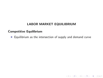
Equilibrium Price Determination Definition 2 An equilibrium price P ∗ is a price at which quantity demanded is equal to quantity supplied. At such price, neither consumers nor suppliers have an incentive to alter their economic decisions. The equilibrium price solves: Q D ( P ∗ , P ′ , I ) = Q S ( P ∗ , v , w ) In the short run the price has two roles: 1) a way to ration demand 2) a signal to producers informing them of how much to produce The equilbrium price changes with the given parameters P ′ , I , v , w . Piacquadio & Traeger: Equilibrium, Welfare, & Information. UiO Spring 2018. 16/27
Shifts in Demand and Supply Curves Demand Curve can shift as a result of changes in: ◮ income, ◮ price of substitutes or complements, ◮ preferences Supply Curve can shift as a result of changes in: ◮ input prices, ◮ number of producers, ◮ technologies The effect of a shift in the demand or supply curve on P ∗ depends on the shape of the two curves. (see blackboard) Piacquadio & Traeger: Equilibrium, Welfare, & Information. UiO Spring 2018. 17/27
Mathematical Model of Market Equilibrium ◮ Demand: Q D = D ( P , α ) where α is a shift-parameter, e.g., income ◮ Supply: Q S = S ( P , β ) where β is a shift-parameter, e.g., price of labor ◮ Equilibrium: Q D = Q S . We will analyze how empirical estimates of the elasticities of demand and supply can help predicting the equilibrium price response of a change in, e.g., income ( α ). Piacquadio & Traeger: Equilibrium, Welfare, & Information. UiO Spring 2018. 18/27
Recommend
More recommend
Explore More Topics
Stay informed with curated content and fresh updates.
