Learning Linear Quadratic Regulators Efficiently with Only - PowerPoint PPT Presentation

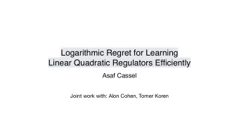
Learning Linear Quadratic Regulators Efficiently with Only Regret T Alon Cohen Joint work with: Tomer Koren and Yishay Mansour

Reinforcement Control Learning Theory Multi-armed Bandits

Linear Quadratic Control Agent Environment

Linear Quadratic Control Control u t ∈ ℝ k Agent Environment x t ∈ ℝ d State

Linear Quadratic Control Control u t ∈ ℝ k Agent Environment x t +1 = A ⋆ x t + B ⋆ u t + w t ∈ ℝ d State w t ∼ 𝒪 ( 0, W ) Noise

Linear Quadratic Control Control u t ∈ ℝ k Agent Environment x t +1 = A ⋆ x t + B ⋆ u t + w t ∈ ℝ d State w t ∼ 𝒪 ( 0, W ) Noise c t = x ⊤ t Qx t + u ⊤ t Ru t Cost

Applications

Planning in LQRs Control u t ∈ ℝ k Agent Environment Policy: π : x t ⟼ u t Optimal policy stabilizes the system in minimum x t +1 = A ⋆ x t + B ⋆ u t + w t ∈ ℝ d cost. State π ⋆ ( x ) = Kx For infinite horizon: c t = x ⊤ t Qx t + u ⊤ t Ru t Cost Dimitri P . Bertsekas, Dynamic Programming and Optimal Control, 2005.

Learning in LQRs Control u t ∈ ℝ k Agent Environment Goal : minimize the regret T T ∑ ∑ R T = cost t ( Alg ) − min cost t ( K ) x t +1 = □ x t + □ u t + w t ∈ ℝ d K t =1 t =1 State c t = x ⊤ t Qx t + u ⊤ t Ru t Abbasi-Yadkori and Szepesvári, 2011 Cost Ibrahimi et al., 2012 Faradonbeh et al., 2017 Ouyang et al., 2017 Abeille and Lazaric, 2017, 2018 Dean et al. 2018, 2019

Our Result First poly-time algorithm for online learning of linear-quadratic control systems with ˜ O ( T ) regret. Resolve an open question of Abbasi-Yadkori and Szepesvári (2011) and Dean, Mania, Matni, Recht, and Tu (2018). Regret E ffi cient

Our Result First poly-time algorithm for online learning of linear-quadratic control systems with ˜ O ( T ) regret. Resolve an open question of Abbasi-Yadkori and Szepesvári (2011) and Dean, Mania, Matni, Recht, and Tu (2018). Regret E ffi cient Abbasi-Yadkori and exp ( d ) T Szepesvári, 2011

Our Result First poly-time algorithm for online learning of linear-quadratic control systems with ˜ O ( T ) regret. Resolve an open question of Abbasi-Yadkori and Szepesvári (2011) and Dean, Mania, Matni, Recht, and Tu (2018). Regret E ffi cient Abbasi-Yadkori and exp ( d ) T Szepesvári, 2011 poly ( d ) Ibrahimi et al., 2012 T

Our Result First poly-time algorithm for online learning of linear-quadratic control systems with ˜ O ( T ) regret. Resolve an open question of Abbasi-Yadkori and Szepesvári (2011) and Dean, Mania, Matni, Recht, and Tu (2018). Regret E ffi cient Abbasi-Yadkori and exp ( d ) T Szepesvári, 2011 poly ( d ) Ibrahimi et al., 2012 T poly ( d ) T 2/3 Dean et al., 2018

Our Result First poly-time algorithm for online learning of linear-quadratic control systems with ˜ O ( T ) regret. Resolve an open question of Abbasi-Yadkori and Szepesvári (2011) and Dean, Mania, Matni, Recht, and Tu (2018). Regret E ffi cient Abbasi-Yadkori and exp ( d ) T Szepesvári, 2011 poly ( d ) Ibrahimi et al., 2012 T poly ( d ) T 2/3 Dean et al., 2018 poly ( d ) Ours T

Our Result First poly-time algorithm for online learning of linear-quadratic control systems with ˜ O ( T ) regret. Resolve an open question of Abbasi-Yadkori and Szepesvári (2011) and Dean, Mania, Matni, Recht, and Tu (2018). Regret E ffi cient Abbasi-Yadkori and exp ( d ) T Szepesvári, 2011 poly ( d ) Ibrahimi et al., 2012 T poly ( d ) T 2/3 Dean et al., 2018 poly ( d ) Ours T * Recent paper by Mania et al., 2019 can be used to derive a result similar to ours.

Solution Techniques Explore-then-Exploit (Dean et al., 2018) Execute + K 0 Gaussian noise u t = K 0 x t + 𝒪 ( 0, ε 2 I )

̂ Solution Techniques Explore-then-Exploit (Dean et al., 2018) ( x t , u t ) T t =1 Execute + Model Estimation K 0 Gaussian noise (Åström, 1968) T ( ̂ ∑ ∥ Ax t + Bu t − x t +1 ∥ 2 u t = K 0 x t + 𝒪 ( 0, ε 2 I ) A B ) = arg min ( A B ) t =1

̂ ̂ ̂ Solution Techniques Explore-then-Exploit (Dean et al., 2018) ( x t , u t ) T ( A B ) t =1 Execute + Model Estimation K 0 Solve Model Gaussian noise (Åström, 1968) T ( ̂ ∑ ∥ Ax t + Bu t − x t +1 ∥ 2 u t = K 0 x t + 𝒪 ( 0, ε 2 I ) A B ) = arg min ( A B ) t =1

̂ ̂ ̂ ̂ Solution Techniques Explore-then-Exploit (Dean et al., 2018) ( x t , u t ) T K ( A B ) t =1 Execute + Model Estimation K 0 Execute Solve Model Gaussian noise (Åström, 1968) T R T = O ( T 2/3 ) ( ̂ ∑ ∥ Ax t + Bu t − x t +1 ∥ 2 u t = K 0 x t + 𝒪 ( 0, ε 2 I ) A B ) = arg min ( A B ) t =1

Solution Techniques B a s e d o n U C R L Optimism in the Face of Uncertainty (Abbasi-Yadkori and Szepesvári, 2011) Θ t ∋ ( A ⋆ B ⋆ )

Solution Techniques B a s e d o n U C R L Optimism in the Face of Uncertainty (Abbasi-Yadkori and Szepesvári, 2011) Θ t ∋ ( A ⋆ B ⋆ ) Find Optimistic Policy π t = arg min J ( A B ) ( π ) π , ( A B ) ∈Θ t

Solution Techniques B a s e d o n U C R L Optimism in the Face of Uncertainty (Abbasi-Yadkori and Szepesvári, 2011) Θ t ∋ ( A ⋆ B ⋆ ) π t Find Optimistic Execute Policy π t = arg min J ( A B ) ( π ) π , ( A B ) ∈Θ t

Solution Techniques B a s e d o n U C R L Optimism in the Face of Uncertainty (Abbasi-Yadkori and Szepesvári, 2011) Θ t ∋ ( A ⋆ B ⋆ ) π t Find Optimistic Execute Policy π t = arg min J ( A B ) ( π ) ( x t , u t ) π , ( A B ) ∈Θ t Update version space

Solution Techniques B a s e d o n U C R L Optimism in the Face of Uncertainty (Abbasi-Yadkori and Szepesvári, 2011) Θ t ∋ ( A ⋆ B ⋆ ) π t Find Optimistic Optimistic in the sense that: Execute Policy J ( A B ) ( π ) ≤ J ( π ⋆ ) . min π t = arg min J ( A B ) ( π ) ( x t , u t ) π , ( A B ) ∈Θ t π , ( A B ) ∈Θ t Update version space R T = O ( T )

Solution Techniques B a s e d o n U C R L Optimism in the Face of Uncertainty (Abbasi-Yadkori and Szepesvári, 2011) Θ t ∋ ( A ⋆ B ⋆ ) π t Find Optimistic Optimistic in the sense that: Execute Policy J ( A B ) ( π ) ≤ J ( π ⋆ ) . min π t = arg min J ( A B ) ( π ) ( x t , u t ) π , ( A B ) ∈Θ t π , ( A B ) ∈Θ t Update version space Caveat : not convex in J ( A B ) ( π ) policy parameters. R T = O ( T )

Convex (SDP) Formulation Cohen et al., 2018 Steady- Σ = 𝔽 [ ( ] . ⊤ state covariance x x u ) ( u ) Convex re-parameterization: matrix LQ Control: Σ = ( Σ xx Σ xu Σ uu ) x t +1 = A ⋆ x t + B ⋆ u t + w t Σ ux c t = x ⊤ t Qx t + u ⊤ t Ru t

Convex (SDP) Formulation Cohen et al., 2018 Steady- Σ = 𝔽 [ ( ] . ⊤ state covariance x x u ) ( u ) Convex re-parameterization: matrix Σ ∙ ( R ) Q 0 min 0 Σ⪰ 0 Σ xx = ( A ⋆ B ⋆ ) Σ ( A ⋆ B ⋆ ) ⊤ + W . s.t. LQ Control: Σ = ( Σ xx Σ xu Σ uu ) Lemma : K = Σ ux Σ − 1 is optimal for LQR. x t +1 = A ⋆ x t + B ⋆ u t + w t xx Σ ux c t = x ⊤ t Qx t + u ⊤ t Ru t

Intuition for Our Algorithm K 1 K 2

Intuition for Our Algorithm K 1 K 2

Intuition for Our Algorithm K 1 K 2 O ( log T )

Intuition for Our Algorithm K 1 K 2 K 3 O ( log T ) O ( log T )

Intuition for Our Algorithm … K 1 K 2 K 3 O ( log T ) O ( log T ) O ( log T ) epochs with high probability. O ( log T ) ˜ T ) regret in total. O (

Intuition for Our Algorithm Warm Start … K 1 K 2 K 3 K 0 ˜ O ( T ) O ( log T ) O ( log T ) O ( log T ) epochs with high probability. O ( log T ) ˜ T ) regret in total. O (

Our Algorithm: OSLO (i) After warm start: F ≤ O ( 1/ T ) . ∥ ( A 0 B 0 ) − ( A ⋆ B ⋆ ) ∥ 2 t − 1 z s = ( V t = λ I + 1 u s ) . x s Maintain: , where ∑ z s z ⊤ s β s =1 Run in epochs: Optimistic Compute using a semidefinite program. K t Execute fixed during epoch. K t Epoch ends when is doubled. det( V t )

Our Algorithm: OSLO (ii) At epoch start: Estimate from past observations A ⋆ , B ⋆ t − 1 1 ∥ ( A B ) z s − x s +1 ∥ 2 + λ ∥ ( A B ) − ( A 0 B 0 ) ∥ 2 ∑ ( A t B t ) = arg min F β ( A B ) s =1 Replaces hard Compute optimistic policy by solving problem in Abbasi-Yadkori & Szepesvári Σ ∙ ( R ) Q 0 Σ t = arg min 0 Σ⪰ 0 Σ xx ⪰ ( A t B t ) Σ ( A t B t ) ⊤ + W − μ ( Σ ∙ V − 1 s.t. t ) I Σ = ( Σ xx Σ xu Σ uu ) K t = ( Σ t ) ux ( Σ t ) − 1 Output: Σ ux xx

Parameter Estimation Lemma (Abbasi-Yadkori and Szepesvari, 2011) tr ( Δ t V t Δ ⊤ Let With high probability t ) ≤ 1. Δ t = ( A t B t ) − ( A ⋆ B ⋆ ) . norm ∥ V t ∥ = Θ ( t ) V t ∥Δ t ∥ = Θ (1/ t ) T Δ t (disregarding switches ∑ “Almost” the regret = ∥Δ t ∥ = O ( T ) t and warm start) t =1

MDP vs. LQR: Boundedness of States Unlike in MDPs states may be unbounded. Low probability if K is stable, but may have unpredictable effect on expectation. System may destabilize when switching between policies too often. Main technique: Generate “sequentially stable” policies. ∥ x t ∥ ⪅ κ w.h.p Keep states bounded with high probability: d log T γ