Hardness of Certification for Constrained PCA Alex Wein Courant - - PowerPoint PPT Presentation

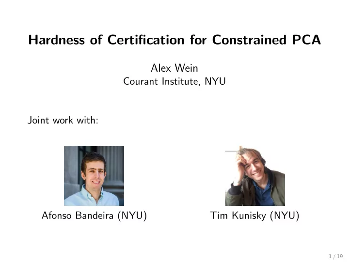
Hardness of Certification for Constrained PCA

Alex Wein

Courant Institute, NYU Joint work with: Afonso Bandeira (NYU) Tim Kunisky (NYU)

1 / 19

Part I: Statistical-to-Computational Gaps and the “Low-Degree Method”

2 / 19

Statistical-to-Computational Gaps

◮ Planted clique: G(n, 1/2) ∪ {k-clique}

3 / 19

Statistical-to-Computational Gaps

◮ Planted clique: G(n, 1/2) ∪ {k-clique}

◮ n vertices 3 / 19

Statistical-to-Computational Gaps

◮ Planted clique: G(n, 1/2) ∪ {k-clique}

◮ n vertices ◮ Each of the

n

2

• edges occurs with probability 1/2

3 / 19

Statistical-to-Computational Gaps

◮ Planted clique: G(n, 1/2) ∪ {k-clique}

◮ n vertices ◮ Each of the

n

2

• edges occurs with probability 1/2

◮ Planted clique on k vertices 3 / 19

Statistical-to-Computational Gaps

◮ Planted clique: G(n, 1/2) ∪ {k-clique}

◮ n vertices ◮ Each of the

n

2

• edges occurs with probability 1/2

◮ Planted clique on k vertices 3 / 19

Statistical-to-Computational Gaps

◮ Planted clique: G(n, 1/2) ∪ {k-clique}

◮ n vertices ◮ Each of the

n

2

• edges occurs with probability 1/2

◮ Planted clique on k vertices ◮ Goal: find the clique 3 / 19

Statistical-to-Computational Gaps

◮ Planted clique: G(n, 1/2) ∪ {k-clique}

4 / 19

Statistical-to-Computational Gaps

◮ Planted clique: G(n, 1/2) ∪ {k-clique}

◮ Statistically, can find planted clique of size (2 + ε) log n 4 / 19

Statistical-to-Computational Gaps

◮ Planted clique: G(n, 1/2) ∪ {k-clique}

◮ Statistically, can find planted clique of size (2 + ε) log n ◮ In poly-time, can only find clique of size Ω(√n) 4 / 19

Statistical-to-Computational Gaps

◮ Planted clique: G(n, 1/2) ∪ {k-clique}

◮ Statistically, can find planted clique of size (2 + ε) log n ◮ In poly-time, can only find clique of size Ω(√n) 4 / 19

Statistical-to-Computational Gaps

◮ Planted clique: G(n, 1/2) ∪ {k-clique}

◮ Statistically, can find planted clique of size (2 + ε) log n ◮ In poly-time, can only find clique of size Ω(√n)

◮ Sparse PCA

4 / 19

Statistical-to-Computational Gaps

◮ Planted clique: G(n, 1/2) ∪ {k-clique}

◮ Statistically, can find planted clique of size (2 + ε) log n ◮ In poly-time, can only find clique of size Ω(√n)

◮ Sparse PCA ◮ Stochastic block model (community detection)

4 / 19

Statistical-to-Computational Gaps

◮ Planted clique: G(n, 1/2) ∪ {k-clique}

◮ Statistically, can find planted clique of size (2 + ε) log n ◮ In poly-time, can only find clique of size Ω(√n)

◮ Sparse PCA ◮ Stochastic block model (community detection) ◮ Random constraint satisfaction problems (e.g. 3-SAT)

4 / 19

Statistical-to-Computational Gaps

◮ Planted clique: G(n, 1/2) ∪ {k-clique}

◮ Statistically, can find planted clique of size (2 + ε) log n ◮ In poly-time, can only find clique of size Ω(√n)

◮ Sparse PCA ◮ Stochastic block model (community detection) ◮ Random constraint satisfaction problems (e.g. 3-SAT) ◮ Tensor PCA

4 / 19

Statistical-to-Computational Gaps

◮ Planted clique: G(n, 1/2) ∪ {k-clique}

◮ Statistically, can find planted clique of size (2 + ε) log n ◮ In poly-time, can only find clique of size Ω(√n)

◮ Sparse PCA ◮ Stochastic block model (community detection) ◮ Random constraint satisfaction problems (e.g. 3-SAT) ◮ Tensor PCA ◮ Tensor decomposition

4 / 19

Statistical-to-Computational Gaps

◮ Planted clique: G(n, 1/2) ∪ {k-clique}

◮ Statistically, can find planted clique of size (2 + ε) log n ◮ In poly-time, can only find clique of size Ω(√n)

◮ Sparse PCA ◮ Stochastic block model (community detection) ◮ Random constraint satisfaction problems (e.g. 3-SAT) ◮ Tensor PCA ◮ Tensor decomposition ◮ Synchronization / orbit recovery

4 / 19

Statistical-to-Computational Gaps

◮ Planted clique: G(n, 1/2) ∪ {k-clique}

◮ Statistically, can find planted clique of size (2 + ε) log n ◮ In poly-time, can only find clique of size Ω(√n)

◮ Sparse PCA ◮ Stochastic block model (community detection) ◮ Random constraint satisfaction problems (e.g. 3-SAT) ◮ Tensor PCA ◮ Tensor decomposition ◮ Synchronization / orbit recovery

Different from theory of NP-completeness: average-case

4 / 19

Statistical-to-Computational Gaps

◮ Planted clique: G(n, 1/2) ∪ {k-clique}

◮ Statistically, can find planted clique of size (2 + ε) log n ◮ In poly-time, can only find clique of size Ω(√n)

◮ Sparse PCA ◮ Stochastic block model (community detection) ◮ Random constraint satisfaction problems (e.g. 3-SAT) ◮ Tensor PCA ◮ Tensor decomposition ◮ Synchronization / orbit recovery

Different from theory of NP-completeness: average-case Q: What fundamentally makes a problem easy or hard?

4 / 19

How to Show that a Problem is Hard?

We don’t know how to prove that average-case problems are hard, but various forms of evidence:

5 / 19

How to Show that a Problem is Hard?

We don’t know how to prove that average-case problems are hard, but various forms of evidence:

◮ Reductions (e.g. from planted clique) [Berthet, Rigollet ’13]

5 / 19

How to Show that a Problem is Hard?

We don’t know how to prove that average-case problems are hard, but various forms of evidence:

◮ Reductions (e.g. from planted clique) [Berthet, Rigollet ’13] ◮ Failure of MCMC [Jerrum ’92]

5 / 19

How to Show that a Problem is Hard?

We don’t know how to prove that average-case problems are hard, but various forms of evidence:

◮ Reductions (e.g. from planted clique) [Berthet, Rigollet ’13] ◮ Failure of MCMC [Jerrum ’92] ◮ Shattering of solution space [Achlioptas, Coja-Oghlan ’08]

5 / 19

How to Show that a Problem is Hard?

We don’t know how to prove that average-case problems are hard, but various forms of evidence:

◮ Reductions (e.g. from planted clique) [Berthet, Rigollet ’13] ◮ Failure of MCMC [Jerrum ’92] ◮ Shattering of solution space [Achlioptas, Coja-Oghlan ’08] ◮ Failure of local algorithms [Gamarnik, Sudan ’13]

5 / 19

How to Show that a Problem is Hard?

We don’t know how to prove that average-case problems are hard, but various forms of evidence:

◮ Reductions (e.g. from planted clique) [Berthet, Rigollet ’13] ◮ Failure of MCMC [Jerrum ’92] ◮ Shattering of solution space [Achlioptas, Coja-Oghlan ’08] ◮ Failure of local algorithms [Gamarnik, Sudan ’13] ◮ Statistical physics, BP [Decelle, Krzakala, Moore, Zdeborov´

a ’11] 5 / 19

How to Show that a Problem is Hard?

We don’t know how to prove that average-case problems are hard, but various forms of evidence:

◮ Reductions (e.g. from planted clique) [Berthet, Rigollet ’13] ◮ Failure of MCMC [Jerrum ’92] ◮ Shattering of solution space [Achlioptas, Coja-Oghlan ’08] ◮ Failure of local algorithms [Gamarnik, Sudan ’13] ◮ Statistical physics, BP [Decelle, Krzakala, Moore, Zdeborov´

a ’11]

◮ Optimization landscape, Kac-Rice [Auffinger, Ben Arous, Cern´

y ’10] 5 / 19

How to Show that a Problem is Hard?

We don’t know how to prove that average-case problems are hard, but various forms of evidence:

◮ Reductions (e.g. from planted clique) [Berthet, Rigollet ’13] ◮ Failure of MCMC [Jerrum ’92] ◮ Shattering of solution space [Achlioptas, Coja-Oghlan ’08] ◮ Failure of local algorithms [Gamarnik, Sudan ’13] ◮ Statistical physics, BP [Decelle, Krzakala, Moore, Zdeborov´

a ’11]

◮ Optimization landscape, Kac-Rice [Auffinger, Ben Arous, Cern´

y ’10]

◮ Sum-of-squares lower bounds [Barak, Hopkins, Kelner, Kothari, Moitra, Potechin ’16]

5 / 19

How to Show that a Problem is Hard?

We don’t know how to prove that average-case problems are hard, but various forms of evidence:

◮ Reductions (e.g. from planted clique) [Berthet, Rigollet ’13] ◮ Failure of MCMC [Jerrum ’92] ◮ Shattering of solution space [Achlioptas, Coja-Oghlan ’08] ◮ Failure of local algorithms [Gamarnik, Sudan ’13] ◮ Statistical physics, BP [Decelle, Krzakala, Moore, Zdeborov´

a ’11]

◮ Optimization landscape, Kac-Rice [Auffinger, Ben Arous, Cern´

y ’10]

◮ Sum-of-squares lower bounds [Barak, Hopkins, Kelner, Kothari, Moitra, Potechin ’16] ◮ This talk: “low-degree method”

[Barak, Hopkins, Kelner, Kothari, Moitra, Potechin ’16; Hopkins, Steurer ’17; Hopkins, Kothari, Potechin, Raghavendra, Schramm, Steurer ’17; Hopkins ’18 (PhD thesis)] 5 / 19

The Low-Degree Method

Suppose we want to hypothesis test (with error probability o(1)) between two distributions:

6 / 19

The Low-Degree Method

Suppose we want to hypothesis test (with error probability o(1)) between two distributions:

◮ Null model Y ∼ Qn

e.g. G(n, 1/2)

6 / 19

The Low-Degree Method

Suppose we want to hypothesis test (with error probability o(1)) between two distributions:

◮ Null model Y ∼ Qn

e.g. G(n, 1/2)

◮ Planted model Y ∼ Pn

e.g. G(n, 1/2) ∪ {k-clique}

6 / 19

The Low-Degree Method

Suppose we want to hypothesis test (with error probability o(1)) between two distributions:

◮ Null model Y ∼ Qn

e.g. G(n, 1/2)

◮ Planted model Y ∼ Pn

e.g. G(n, 1/2) ∪ {k-clique}

Look for a degree-D multivariate polynomial f that distinguishes P from Q: max

f ∈R[Y ]D

EY ∼P[f (Y )]

• EY ∼Q[f (Y )2]

6 / 19

The Low-Degree Method

Suppose we want to hypothesis test (with error probability o(1)) between two distributions:

◮ Null model Y ∼ Qn

e.g. G(n, 1/2)

◮ Planted model Y ∼ Pn

e.g. G(n, 1/2) ∪ {k-clique}

Look for a degree-D multivariate polynomial f that distinguishes P from Q: max

f ∈R[Y ]D

EY ∼P[f (Y )]

• EY ∼Q[f (Y )2]

Want f (Y ) to be big when Y ∼ P and small when Y ∼ Q

6 / 19

The Low-Degree Method

max

f ∈R[Y ]D

EY ∼P[f (Y )]

• EY ∼Q[f (Y )2]

R[Y ]D: polynomials of degree ≤ D (subspace)

7 / 19

The Low-Degree Method

max

f ∈R[Y ]D

EY ∼P[f (Y )]

• EY ∼Q[f (Y )2]

= max

f ∈R[Y ]D

EY ∼Q[L(Y )f (Y )]

• EY ∼Q[f (Y )2]

R[Y ]D: polynomials of degree ≤ D (subspace) L(Y ) = dP

dQ(Y )

7 / 19

The Low-Degree Method

max

f ∈R[Y ]D

EY ∼P[f (Y )]

• EY ∼Q[f (Y )2]

= max

f ∈R[Y ]D

EY ∼Q[L(Y )f (Y )]

• EY ∼Q[f (Y )2]

= max

f ∈R[Y ]D

L, f f R[Y ]D: polynomials of degree ≤ D (subspace) L(Y ) = dP

dQ(Y )

f , g = EY ∼Q[f (Y )g(Y )] f =

• f , f

7 / 19

The Low-Degree Method

max

f ∈R[Y ]D

EY ∼P[f (Y )]

• EY ∼Q[f (Y )2]

= max

f ∈R[Y ]D

EY ∼Q[L(Y )f (Y )]

• EY ∼Q[f (Y )2]

= max

f ∈R[Y ]D

L, f f = L≤D R[Y ]D: polynomials of degree ≤ D (subspace) L(Y ) = dP

dQ(Y )

f , g = EY ∼Q[f (Y )g(Y )] f =

• f , f

Maximizer: f = L≤D := proj(R[Y ]D)L

7 / 19

The Low-Degree Method

max

f ∈R[Y ]D

EY ∼P[f (Y )]

• EY ∼Q[f (Y )2]

= max

f ∈R[Y ]D

EY ∼Q[L(Y )f (Y )]

• EY ∼Q[f (Y )2]

= max

f ∈R[Y ]D

L, f f = L≤D R[Y ]D: polynomials of degree ≤ D (subspace) L(Y ) = dP

dQ(Y )

f , g = EY ∼Q[f (Y )g(Y )] f =

• f , f

Maximizer: f = L≤D := proj(R[Y ]D)L Norm of low-degree likelihood ratio

7 / 19

The Low-Degree Method

Conclusion: maxf ∈R[Y ]D

EY ∼P[f (Y )]

√

EY ∼Q[f (Y )2] = L≤D

8 / 19

The Low-Degree Method

Conclusion: maxf ∈R[Y ]D

EY ∼P[f (Y )]

√

EY ∼Q[f (Y )2] = L≤D

Heuristically, L≤D = ω(1) degree-D polynomial can distinguish Q, P O(1) degree-D polynomials fail

8 / 19

The Low-Degree Method

Conclusion: maxf ∈R[Y ]D

EY ∼P[f (Y )]

√

EY ∼Q[f (Y )2] = L≤D

Heuristically, L≤D = ω(1) degree-D polynomial can distinguish Q, P O(1) degree-D polynomials fail Degree-O(log n) polynomials ⇔ Polynomial-time algorithms

8 / 19

The Low-Degree Method

Conclusion: maxf ∈R[Y ]D

EY ∼P[f (Y )]

√

EY ∼Q[f (Y )2] = L≤D

Heuristically, L≤D = ω(1) degree-D polynomial can distinguish Q, P O(1) degree-D polynomials fail Degree-O(log n) polynomials ⇔ Polynomial-time algorithms

◮ Spectral method: distinguish via top eigenvalue of matrix

M = M(Y ) whose entries are O(1)-degree polynomials in Y

8 / 19

The Low-Degree Method

Conclusion: maxf ∈R[Y ]D

EY ∼P[f (Y )]

√

EY ∼Q[f (Y )2] = L≤D

Heuristically, L≤D = ω(1) degree-D polynomial can distinguish Q, P O(1) degree-D polynomials fail Degree-O(log n) polynomials ⇔ Polynomial-time algorithms

◮ Spectral method: distinguish via top eigenvalue of matrix

M = M(Y ) whose entries are O(1)-degree polynomials in Y

◮ Log-degree distinguisher: f (Y ) = Tr(Mq) with q = Θ(log n)

8 / 19

The Low-Degree Method

Conclusion: maxf ∈R[Y ]D

EY ∼P[f (Y )]

√

EY ∼Q[f (Y )2] = L≤D

Heuristically, L≤D = ω(1) degree-D polynomial can distinguish Q, P O(1) degree-D polynomials fail Degree-O(log n) polynomials ⇔ Polynomial-time algorithms

◮ Spectral method: distinguish via top eigenvalue of matrix

M = M(Y ) whose entries are O(1)-degree polynomials in Y

◮ Log-degree distinguisher: f (Y ) = Tr(Mq) with q = Θ(log n) ◮ Spectral methods ⇔ sum-of-squares [HKPRSS ’17]

8 / 19

The Low-Degree Method

Conclusion: maxf ∈R[Y ]D

EY ∼P[f (Y )]

√

EY ∼Q[f (Y )2] = L≤D

Heuristically, L≤D = ω(1) degree-D polynomial can distinguish Q, P O(1) degree-D polynomials fail Degree-O(log n) polynomials ⇔ Polynomial-time algorithms

◮ Spectral method: distinguish via top eigenvalue of matrix

M = M(Y ) whose entries are O(1)-degree polynomials in Y

◮ Log-degree distinguisher: f (Y ) = Tr(Mq) with q = Θ(log n) ◮ Spectral methods ⇔ sum-of-squares [HKPRSS ’17]

Conjecture (informal variant of [Hopkins ’18])

For “nice” Q, P, if L≤D = O(1) for D = log1+Ω(1)(n) then no polynomial-time algorithm can distinguish Q, P with success probability 1 − o(1).

8 / 19

Advantages of the Low-Degree Method

◮ Can actually calculate/bound L≤D for many problems

9 / 19

Advantages of the Low-Degree Method

◮ Can actually calculate/bound L≤D for many problems ◮ And the predictions are correct! (i.e. matching widely-believed

conjectures)

9 / 19

Advantages of the Low-Degree Method

◮ Can actually calculate/bound L≤D for many problems ◮ And the predictions are correct! (i.e. matching widely-believed

conjectures)

◮ Planted clique, sparse PCA, stochastic block model, tensor

PCA, ...

9 / 19

Advantages of the Low-Degree Method

◮ Can actually calculate/bound L≤D for many problems ◮ And the predictions are correct! (i.e. matching widely-believed

conjectures)

◮ Planted clique, sparse PCA, stochastic block model, tensor

PCA, ...

◮ Heuristically, low-degree prediction matches performance of

sum-of-squares

9 / 19

Advantages of the Low-Degree Method

◮ Can actually calculate/bound L≤D for many problems ◮ And the predictions are correct! (i.e. matching widely-believed

conjectures)

◮ Planted clique, sparse PCA, stochastic block model, tensor

PCA, ...

◮ Heuristically, low-degree prediction matches performance of

sum-of-squares

◮ But low-degree calculation is much easier than proving SOS

lower bounds

9 / 19

Advantages of the Low-Degree Method

◮ Can actually calculate/bound L≤D for many problems ◮ And the predictions are correct! (i.e. matching widely-believed

conjectures)

◮ Planted clique, sparse PCA, stochastic block model, tensor

PCA, ...

◮ Heuristically, low-degree prediction matches performance of

sum-of-squares

◮ But low-degree calculation is much easier than proving SOS

lower bounds

◮ By varying degree D, can explore power of

subexponential-time algorithms:

◮ Degree-nδ polynomials ⇔ Time-2nδ algorithms

δ ∈ (0, 1)

9 / 19

How to Compute L≤D

Additive Gaussian noise: P : Y = X + Z vs Q : Y = Z where X ∼ P, any distribution over RN and Z is i.i.d. N(0, 1)

10 / 19

How to Compute L≤D

Additive Gaussian noise: P : Y = X + Z vs Q : Y = Z where X ∼ P, any distribution over RN and Z is i.i.d. N(0, 1) L(Y ) = dP dQ(Y ) = EX exp(− 1

2Y − X2)

exp(− 1

2Y 2)

= EX exp(Y , X−1 2X2)

10 / 19

How to Compute L≤D

Additive Gaussian noise: P : Y = X + Z vs Q : Y = Z where X ∼ P, any distribution over RN and Z is i.i.d. N(0, 1) L(Y ) = dP dQ(Y ) = EX exp(− 1

2Y − X2)

exp(− 1

2Y 2)

= EX exp(Y , X−1 2X2) Write L =

α cαhα where {hα} are Hermite polynomials

(orthonormal basis w.r.t. Q)

10 / 19

How to Compute L≤D

Additive Gaussian noise: P : Y = X + Z vs Q : Y = Z where X ∼ P, any distribution over RN and Z is i.i.d. N(0, 1) L(Y ) = dP dQ(Y ) = EX exp(− 1

2Y − X2)

exp(− 1

2Y 2)

= EX exp(Y , X−1 2X2) Write L =

α cαhα where {hα} are Hermite polynomials

(orthonormal basis w.r.t. Q)

L≤D2 =

|α|≤D c2 α where cα = L, hα = EY ∼Q[L(Y )hα(Y )]

10 / 19

How to Compute L≤D

Additive Gaussian noise: P : Y = X + Z vs Q : Y = Z where X ∼ P, any distribution over RN and Z is i.i.d. N(0, 1) L(Y ) = dP dQ(Y ) = EX exp(− 1

2Y − X2)

exp(− 1

2Y 2)

= EX exp(Y , X−1 2X2) Write L =

α cαhα where {hα} are Hermite polynomials

(orthonormal basis w.r.t. Q)

L≤D2 =

|α|≤D c2 α where cα = L, hα = EY ∼Q[L(Y )hα(Y )]

· · ·

10 / 19

How to Compute L≤D

Additive Gaussian noise: P : Y = X + Z vs Q : Y = Z where X ∼ P, any distribution over RN and Z is i.i.d. N(0, 1) L(Y ) = dP dQ(Y ) = EX exp(− 1

2Y − X2)

exp(− 1

2Y 2)

= EX exp(Y , X−1 2X2) Write L =

α cαhα where {hα} are Hermite polynomials

(orthonormal basis w.r.t. Q)

L≤D2 =

|α|≤D c2 α where cα = L, hα = EY ∼Q[L(Y )hα(Y )]

· · · Result: L≤D2 = D

d=0 1 d!EX,X ′[X, X ′d]

10 / 19

Part II: Hardness of Certification for Constrained PCA Problems

11 / 19

Constrained PCA

Let W ∼ GOE(n) “Gaussian orthogonal ensemble”

◮ n × n random symmetric matrix:

Wij = Wji ∼ N(0, 1/n), Wii ∼ N(0, 2/n)

12 / 19

Constrained PCA

Let W ∼ GOE(n) “Gaussian orthogonal ensemble”

◮ n × n random symmetric matrix:

Wij = Wji ∼ N(0, 1/n), Wii ∼ N(0, 2/n)

◮ Eigenvalues follow semicircle law on [−2, 2]

12 / 19

Constrained PCA

Let W ∼ GOE(n) “Gaussian orthogonal ensemble”

◮ n × n random symmetric matrix:

Wij = Wji ∼ N(0, 1/n), Wii ∼ N(0, 2/n)

◮ Eigenvalues follow semicircle law on [−2, 2]

PCA: max

x=1 x⊤Wx

12 / 19

Constrained PCA

Let W ∼ GOE(n) “Gaussian orthogonal ensemble”

◮ n × n random symmetric matrix:

Wij = Wji ∼ N(0, 1/n), Wii ∼ N(0, 2/n)

◮ Eigenvalues follow semicircle law on [−2, 2]

PCA: max

x=1 x⊤Wx = λmax(W ) → 2

as n → ∞

12 / 19

Constrained PCA

Let W ∼ GOE(n) “Gaussian orthogonal ensemble”

◮ n × n random symmetric matrix:

Wij = Wji ∼ N(0, 1/n), Wii ∼ N(0, 2/n)

◮ Eigenvalues follow semicircle law on [−2, 2]

PCA: max

x=1 x⊤Wx = λmax(W ) → 2

as n → ∞ Constrained PCA: φ(W ) := max

x∈{±1/√n}n x⊤Wx

12 / 19

Constrained PCA

Let W ∼ GOE(n) “Gaussian orthogonal ensemble”

◮ n × n random symmetric matrix:

Wij = Wji ∼ N(0, 1/n), Wii ∼ N(0, 2/n)

◮ Eigenvalues follow semicircle law on [−2, 2]

PCA: max

x=1 x⊤Wx = λmax(W ) → 2

as n → ∞ Constrained PCA: φ(W ) := max

x∈{±1/√n}n x⊤Wx

Statistical physics: “Sherrington–Kirkpatrick spin glass model”

◮ φ(W ) → 2P∗ ≈ 1.5264 as n → ∞ [Parisi ’80; Talagrand ’06]

12 / 19

Search vs Certification

φ(W ) := max

x∈{±1/√n}n x⊤Wx,

W ∼ GOE(n)

13 / 19

Search vs Certification

φ(W ) := max

x∈{±1/√n}n x⊤Wx,

W ∼ GOE(n) Two computational problems:

13 / 19

Search vs Certification

φ(W ) := max

x∈{±1/√n}n x⊤Wx,

W ∼ GOE(n) Two computational problems:

◮ Search: given W , find x ∈ {±1/√n}n with large x⊤Wx

13 / 19

Search vs Certification

φ(W ) := max

x∈{±1/√n}n x⊤Wx,

W ∼ GOE(n) Two computational problems:

◮ Search: given W , find x ∈ {±1/√n}n with large x⊤Wx

◮ Proves a lower bound on φ(W ) 13 / 19

Search vs Certification

φ(W ) := max

x∈{±1/√n}n x⊤Wx,

W ∼ GOE(n) Two computational problems:

◮ Search: given W , find x ∈ {±1/√n}n with large x⊤Wx

◮ Proves a lower bound on φ(W )

◮ Certification: given W , prove φ(W ) ≤ B for some bound B

13 / 19

Search vs Certification

φ(W ) := max

x∈{±1/√n}n x⊤Wx,

W ∼ GOE(n) Two computational problems:

◮ Search: given W , find x ∈ {±1/√n}n with large x⊤Wx

◮ Proves a lower bound on φ(W )

◮ Certification: given W , prove φ(W ) ≤ B for some bound B

◮ Formally: algorithm {fn} outputs fn(W ) ∈ R such that: 13 / 19

Search vs Certification

φ(W ) := max

x∈{±1/√n}n x⊤Wx,

W ∼ GOE(n) Two computational problems:

◮ Search: given W , find x ∈ {±1/√n}n with large x⊤Wx

◮ Proves a lower bound on φ(W )

◮ Certification: given W , prove φ(W ) ≤ B for some bound B

◮ Formally: algorithm {fn} outputs fn(W ) ∈ R such that:

(i) φ(W ) ≤ fn(W ) ∀W ∈ Rn×n

13 / 19

Search vs Certification

φ(W ) := max

x∈{±1/√n}n x⊤Wx,

W ∼ GOE(n) Two computational problems:

◮ Search: given W , find x ∈ {±1/√n}n with large x⊤Wx

◮ Proves a lower bound on φ(W )

◮ Certification: given W , prove φ(W ) ≤ B for some bound B

◮ Formally: algorithm {fn} outputs fn(W ) ∈ R such that:

(i) φ(W ) ≤ fn(W ) ∀W ∈ Rn×n (ii) if W ∼ GOE(n), fn(W ) ≤ B + o(1) w.p. 1 − o(1)

13 / 19

Search vs Certification

φ(W ) := max

x∈{±1/√n}n x⊤Wx,

W ∼ GOE(n) Two computational problems:

◮ Search: given W , find x ∈ {±1/√n}n with large x⊤Wx

◮ Proves a lower bound on φ(W )

◮ Certification: given W , prove φ(W ) ≤ B for some bound B

◮ Formally: algorithm {fn} outputs fn(W ) ∈ R such that:

(i) φ(W ) ≤ fn(W ) ∀W ∈ Rn×n (ii) if W ∼ GOE(n), fn(W ) ≤ B + o(1) w.p. 1 − o(1)

◮ Note: cannot just output fn(W ) = 2P∗ + ε 13 / 19

Search vs Certification

φ(W ) := max

x∈{±1/√n}n x⊤Wx,

W ∼ GOE(n) Two computational problems:

◮ Search: given W , find x ∈ {±1/√n}n with large x⊤Wx

◮ Proves a lower bound on φ(W )

◮ Certification: given W , prove φ(W ) ≤ B for some bound B

◮ Formally: algorithm {fn} outputs fn(W ) ∈ R such that:

(i) φ(W ) ≤ fn(W ) ∀W ∈ Rn×n (ii) if W ∼ GOE(n), fn(W ) ≤ B + o(1) w.p. 1 − o(1)

◮ Note: cannot just output fn(W ) = 2P∗ + ε 13 / 19

Search vs Certification: Prior Work

14 / 19

Search vs Certification: Prior Work

Perfect search is possible in poly time

14 / 19

Search vs Certification: Prior Work

Perfect search is possible in poly time

◮ Can find x ∈ {±1/√n}n such that x⊤Wx ≥ 2P∗ − ε [Montanari ’18]

14 / 19

Search vs Certification: Prior Work

Perfect search is possible in poly time

◮ Can find x ∈ {±1/√n}n such that x⊤Wx ≥ 2P∗ − ε [Montanari ’18] ◮ Optimization of full-RSB models [Subag ’18]

14 / 19

Search vs Certification: Prior Work

Perfect search is possible in poly time

◮ Can find x ∈ {±1/√n}n such that x⊤Wx ≥ 2P∗ − ε [Montanari ’18] ◮ Optimization of full-RSB models [Subag ’18]

Trivial spectral certification:

14 / 19

Search vs Certification: Prior Work

Perfect search is possible in poly time

◮ Can find x ∈ {±1/√n}n such that x⊤Wx ≥ 2P∗ − ε [Montanari ’18] ◮ Optimization of full-RSB models [Subag ’18]

Trivial spectral certification: φ(W ) ≤ max

x=1 x⊤Wx = λmax(W ) → 2

14 / 19

Search vs Certification: Prior Work

Perfect search is possible in poly time

◮ Can find x ∈ {±1/√n}n such that x⊤Wx ≥ 2P∗ − ε [Montanari ’18] ◮ Optimization of full-RSB models [Subag ’18]

Trivial spectral certification: φ(W ) ≤ max

x=1 x⊤Wx = λmax(W ) → 2

Can we do better (in poly time)?

14 / 19

Search vs Certification: Prior Work

Perfect search is possible in poly time

◮ Can find x ∈ {±1/√n}n such that x⊤Wx ≥ 2P∗ − ε [Montanari ’18] ◮ Optimization of full-RSB models [Subag ’18]

Trivial spectral certification: φ(W ) ≤ max

x=1 x⊤Wx = λmax(W ) → 2

Can we do better (in poly time)?

◮ Convex relaxation?

14 / 19

Search vs Certification: Prior Work

Perfect search is possible in poly time

◮ Can find x ∈ {±1/√n}n such that x⊤Wx ≥ 2P∗ − ε [Montanari ’18] ◮ Optimization of full-RSB models [Subag ’18]

Trivial spectral certification: φ(W ) ≤ max

x=1 x⊤Wx = λmax(W ) → 2

Can we do better (in poly time)?

◮ Convex relaxation? ◮ Sum-of-squares?

14 / 19

Search vs Certification: Prior Work

Perfect search is possible in poly time

◮ Can find x ∈ {±1/√n}n such that x⊤Wx ≥ 2P∗ − ε [Montanari ’18] ◮ Optimization of full-RSB models [Subag ’18]

Trivial spectral certification: φ(W ) ≤ max

x=1 x⊤Wx = λmax(W ) → 2

Can we do better (in poly time)?

◮ Convex relaxation? ◮ Sum-of-squares?

Answer: no!

14 / 19

Search vs Certification: Prior Work

Perfect search is possible in poly time

◮ Can find x ∈ {±1/√n}n such that x⊤Wx ≥ 2P∗ − ε [Montanari ’18] ◮ Optimization of full-RSB models [Subag ’18]

Trivial spectral certification: φ(W ) ≤ max

x=1 x⊤Wx = λmax(W ) → 2

Can we do better (in poly time)?

◮ Convex relaxation? ◮ Sum-of-squares?

Answer: no!

◮ In particular, any convex relaxation fails

14 / 19

Search vs Certification: Prior Work

Perfect search is possible in poly time

◮ Can find x ∈ {±1/√n}n such that x⊤Wx ≥ 2P∗ − ε [Montanari ’18] ◮ Optimization of full-RSB models [Subag ’18]

Trivial spectral certification: φ(W ) ≤ max

x=1 x⊤Wx = λmax(W ) → 2

Can we do better (in poly time)?

◮ Convex relaxation? ◮ Sum-of-squares?

Answer: no!

◮ In particular, any convex relaxation fails

14 / 19

Main Result

15 / 19

Main Result

Theorem (informal)

Conditional on the low-degree method, for any ε > 0, no polynomial-time algorithm can certify an upper bound of 2 − ε on φ(W ).

15 / 19

Main Result

Theorem (informal)

Conditional on the low-degree method, for any ε > 0, no polynomial-time algorithm can certify an upper bound of 2 − ε on φ(W ).

◮ In fact, need essentially exponential time: 2n1−o(1)

15 / 19

Main Result

Theorem (informal)

Conditional on the low-degree method, for any ε > 0, no polynomial-time algorithm can certify an upper bound of 2 − ε on φ(W ).

◮ In fact, need essentially exponential time: 2n1−o(1) ◮ Also for constraint sets other than {±1/√n}n

15 / 19

Main Result

Theorem (informal)

Conditional on the low-degree method, for any ε > 0, no polynomial-time algorithm can certify an upper bound of 2 − ε on φ(W ).

◮ In fact, need essentially exponential time: 2n1−o(1) ◮ Also for constraint sets other than {±1/√n}n

Proof outline:

15 / 19

Main Result

Theorem (informal)

Conditional on the low-degree method, for any ε > 0, no polynomial-time algorithm can certify an upper bound of 2 − ε on φ(W ).

◮ In fact, need essentially exponential time: 2n1−o(1) ◮ Also for constraint sets other than {±1/√n}n

Proof outline: (i) Reduction from a hypothesis testing problem (negatively-spiked Wishart) to certification problem

15 / 19

Main Result

Theorem (informal)

Conditional on the low-degree method, for any ε > 0, no polynomial-time algorithm can certify an upper bound of 2 − ε on φ(W ).

◮ In fact, need essentially exponential time: 2n1−o(1) ◮ Also for constraint sets other than {±1/√n}n

Proof outline: (i) Reduction from a hypothesis testing problem (negatively-spiked Wishart) to certification problem (ii) Use low-degree method to show that the hypothesis testing problem is hard

15 / 19

Spiked Wishart Model

16 / 19

Spiked Wishart Model

Q : Observe N independent samples y1, . . . , yN where yi ∼ N(0, In)

16 / 19

Spiked Wishart Model

Q : Observe N independent samples y1, . . . , yN where yi ∼ N(0, In) P : Planted vector x ∼ Unif({±1/√n}n) Observe y1, . . . , yN with yi ∼ N(0, In + βxx⊤) Parameters: n/N → γ, β ∈ [−1, ∞)

16 / 19

Spiked Wishart Model

Q : Observe N independent samples y1, . . . , yN where yi ∼ N(0, In) P : Planted vector x ∼ Unif({±1/√n}n) Observe y1, . . . , yN with yi ∼ N(0, In + βxx⊤) Parameters: n/N → γ, β ∈ [−1, ∞) Spectral threshold: if β2 > γ, can distinguish Q, P using top/bottom eigenvalue of sample covariance matrix Y = 1

N

• i yiy⊤

i

[Baik, Ben Arous, P´ ech´ e ’05] 16 / 19

Spiked Wishart Model

Q : Observe N independent samples y1, . . . , yN where yi ∼ N(0, In) P : Planted vector x ∼ Unif({±1/√n}n) Observe y1, . . . , yN with yi ∼ N(0, In + βxx⊤) Parameters: n/N → γ, β ∈ [−1, ∞) Spectral threshold: if β2 > γ, can distinguish Q, P using top/bottom eigenvalue of sample covariance matrix Y = 1

N

• i yiy⊤

i

[Baik, Ben Arous, P´ ech´ e ’05]

Using low-degree method, we show: if β2 < γ, cannot distinguish Q, P (unless given exponential time)

16 / 19

Negatively-Spiked Wishart Model

Our case of interest: β = −1 (technically β > −1, β ≈ −1)

17 / 19

Negatively-Spiked Wishart Model

Our case of interest: β = −1 (technically β > −1, β ≈ −1) Q : observe N random vectors in Rn

17 / 19

Negatively-Spiked Wishart Model

Our case of interest: β = −1 (technically β > −1, β ≈ −1) Q : observe N random vectors in Rn P : observe N random vectors that are all orthogonal to a planted hypercube vector x ∈ {±1/√n}n

◮ yi ∼ N(0, In − xx⊤)

17 / 19

Negatively-Spiked Wishart Model

Our case of interest: β = −1 (technically β > −1, β ≈ −1) Q : observe N random vectors in Rn P : observe N random vectors that are all orthogonal to a planted hypercube vector x ∈ {±1/√n}n

◮ yi ∼ N(0, In − xx⊤)

Spectral threshold: if N ≥ n, can distinguish using rank(y1, . . . , yN)

◮ Q: rank n ◮ P: rank n − 1

17 / 19

Negatively-Spiked Wishart Model

Our case of interest: β = −1 (technically β > −1, β ≈ −1) Q : observe N random vectors in Rn P : observe N random vectors that are all orthogonal to a planted hypercube vector x ∈ {±1/√n}n

◮ yi ∼ N(0, In − xx⊤)

Spectral threshold: if N ≥ n, can distinguish using rank(y1, . . . , yN)

◮ Q: rank n ◮ P: rank n − 1

Low-degree method: if N < n, cannot distinguish (unless given exponential time)

17 / 19

Negatively-Spiked Wishart Model

Our case of interest: β = −1 (technically β > −1, β ≈ −1) Q : observe N random vectors in Rn P : observe N random vectors that are all orthogonal to a planted hypercube vector x ∈ {±1/√n}n

◮ yi ∼ N(0, In − xx⊤)

Spectral threshold: if N ≥ n, can distinguish using rank(y1, . . . , yN)

◮ Q: rank n ◮ P: rank n − 1

Low-degree method: if N < n, cannot distinguish (unless given exponential time)

◮ But statistically possible

17 / 19

Reduction from Wishart to Certification

◮ Suppose you can certify φ(W ) ≤ 2 − ε when W ∼ GOE(n)

◮ Recall φ(W ) = maxx∈{±1/√n}n x⊤Wx 18 / 19

Reduction from Wishart to Certification

◮ Suppose you can certify φ(W ) ≤ 2 − ε when W ∼ GOE(n)

◮ Recall φ(W ) = maxx∈{±1/√n}n x⊤Wx

◮ Then you can certify that the top δn-dimensional eigenspace

• f W does not contain a hypercube vector

◮ If hypercube vector x is a linear combination of the top δn

eigenvectors, it would satisfy x⊤Wx ≥ 2 − ε

18 / 19

Reduction from Wishart to Certification

◮ Suppose you can certify φ(W ) ≤ 2 − ε when W ∼ GOE(n)

◮ Recall φ(W ) = maxx∈{±1/√n}n x⊤Wx

◮ Then you can certify that the top δn-dimensional eigenspace

• f W does not contain a hypercube vector

18 / 19

Reduction from Wishart to Certification

◮ Suppose you can certify φ(W ) ≤ 2 − ε when W ∼ GOE(n)

◮ Recall φ(W ) = maxx∈{±1/√n}n x⊤Wx

◮ Then you can certify that the top δn-dimensional eigenspace

• f W does not contain a hypercube vector

◮ So you can certify that a random δn-dimensional subspace

does not contain a hypercube vector

18 / 19

Reduction from Wishart to Certification

◮ Suppose you can certify φ(W ) ≤ 2 − ε when W ∼ GOE(n)

◮ Recall φ(W ) = maxx∈{±1/√n}n x⊤Wx

◮ Then you can certify that the top δn-dimensional eigenspace

• f W does not contain a hypercube vector

◮ So you can certify that a random δn-dimensional subspace

does not contain a hypercube vector

◮ So you can distinguish between a random δn-dimensional

subspace and a δn-dimensional subspace containing a hypercube vector

18 / 19

Reduction from Wishart to Certification

◮ Suppose you can certify φ(W ) ≤ 2 − ε when W ∼ GOE(n)

◮ Recall φ(W ) = maxx∈{±1/√n}n x⊤Wx

◮ Then you can certify that the top δn-dimensional eigenspace

• f W does not contain a hypercube vector

◮ So you can certify that a random δn-dimensional subspace

does not contain a hypercube vector

◮ So you can distinguish between a random δn-dimensional

subspace and a δn-dimensional subspace containing a hypercube vector

◮ So you can distinguish between a random

(1 − δ)n-dimensional subspace and a (1 − δ)n-dimensional subspace that is orthogonal to a hypercube vector

18 / 19

Reduction from Wishart to Certification

◮ Suppose you can certify φ(W ) ≤ 2 − ε when W ∼ GOE(n)

◮ Recall φ(W ) = maxx∈{±1/√n}n x⊤Wx

◮ Then you can certify that the top δn-dimensional eigenspace

• f W does not contain a hypercube vector

◮ So you can certify that a random δn-dimensional subspace

does not contain a hypercube vector

◮ So you can distinguish between a random δn-dimensional

subspace and a δn-dimensional subspace containing a hypercube vector

◮ So you can distinguish between a random

(1 − δ)n-dimensional subspace and a (1 − δ)n-dimensional subspace that is orthogonal to a hypercube vector

◮ But this is exactly the Wishart problem with β = −1 and

N = (1 − δ)n, which is hard ⇒ contradiction

18 / 19

Summary

19 / 19

Summary

◮ Low-degree method: systematic way to predict when

hypothesis testing problems are computationally easy/hard

19 / 19

Summary

◮ Low-degree method: systematic way to predict when

hypothesis testing problems are computationally easy/hard

◮ But what about other types of average-case problems?

19 / 19

Summary

◮ Low-degree method: systematic way to predict when

hypothesis testing problems are computationally easy/hard

◮ But what about other types of average-case problems?

◮ Search 19 / 19

Summary

◮ Low-degree method: systematic way to predict when

hypothesis testing problems are computationally easy/hard

◮ But what about other types of average-case problems?

◮ Search ◮ Certification 19 / 19

Summary

◮ Low-degree method: systematic way to predict when

hypothesis testing problems are computationally easy/hard

◮ But what about other types of average-case problems?

◮ Search ◮ Certification ◮ Recovery (e.g. tensor decomposition) 19 / 19

Summary

◮ Low-degree method: systematic way to predict when

hypothesis testing problems are computationally easy/hard

◮ But what about other types of average-case problems?

◮ Search ◮ Certification ◮ Recovery (e.g. tensor decomposition) ◮ Sampling 19 / 19

Summary

◮ Low-degree method: systematic way to predict when

hypothesis testing problems are computationally easy/hard

◮ But what about other types of average-case problems?

◮ Search ◮ Certification ◮ Recovery (e.g. tensor decomposition) ◮ Sampling ◮ Counting solutions 19 / 19

Summary

◮ Low-degree method: systematic way to predict when

hypothesis testing problems are computationally easy/hard

◮ But what about other types of average-case problems?

◮ Search ◮ Certification ◮ Recovery (e.g. tensor decomposition) ◮ Sampling ◮ Counting solutions

◮ For constrained PCA, we gave low-degree evidence that

certification is hard by reduction from a hypothesis testing problem (negatively-spiked Wishart)

19 / 19

Summary

◮ Low-degree method: systematic way to predict when

hypothesis testing problems are computationally easy/hard

◮ But what about other types of average-case problems?

◮ Search ◮ Certification ◮ Recovery (e.g. tensor decomposition) ◮ Sampling ◮ Counting solutions

◮ For constrained PCA, we gave low-degree evidence that

certification is hard by reduction from a hypothesis testing problem (negatively-spiked Wishart)

◮ Future direction: how to systematically predict hardness for

• ther types of certification/search/etc problems?

19 / 19

Summary

◮ Low-degree method: systematic way to predict when

hypothesis testing problems are computationally easy/hard

◮ But what about other types of average-case problems?

◮ Search ◮ Certification ◮ Recovery (e.g. tensor decomposition) ◮ Sampling ◮ Counting solutions

◮ For constrained PCA, we gave low-degree evidence that

certification is hard by reduction from a hypothesis testing problem (negatively-spiked Wishart)

◮ Future direction: how to systematically predict hardness for

• ther types of certification/search/etc problems?

Thanks!

19 / 19