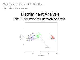
Discriminant Analysis Aleix M. Martinez aleix@ece.osu.edu PCA - PDF document
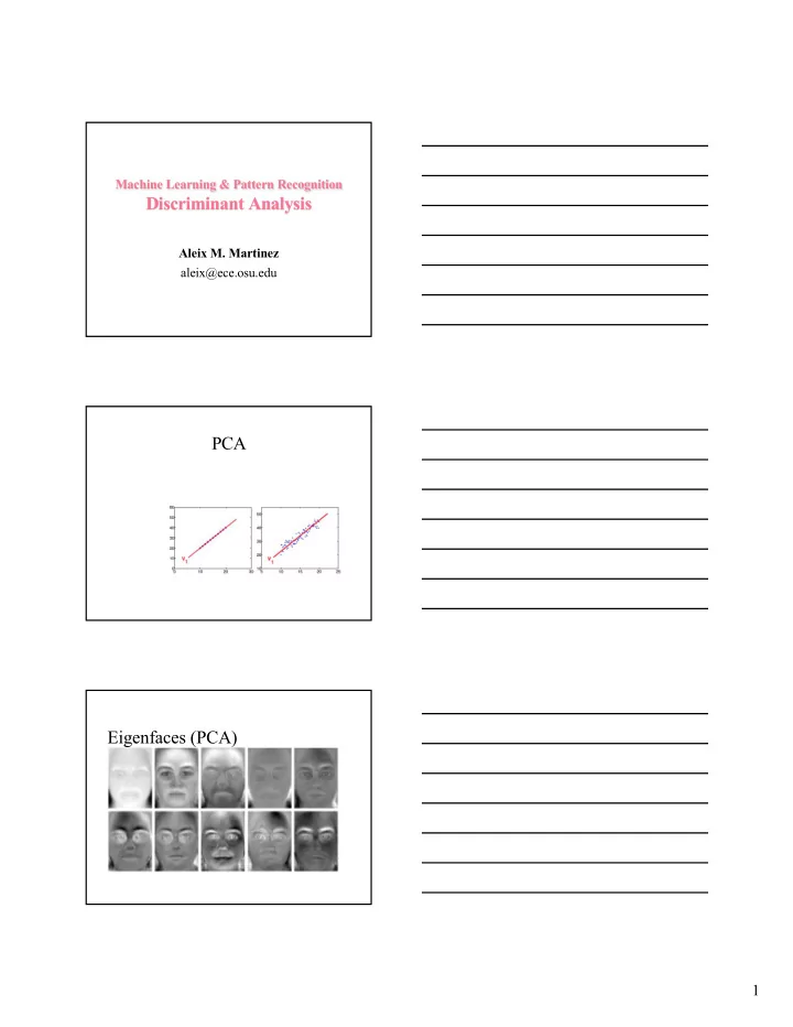
Machine Learning & Pattern Recognition Discriminant Analysis Aleix M. Martinez aleix@ece.osu.edu PCA Eigenfaces (PCA) 1 Linear Discriminant Analysis If we have samples corresponding to two or more classes, we prefer to select those
Machine Learning & Pattern Recognition Discriminant Analysis Aleix M. Martinez aleix@ece.osu.edu PCA Eigenfaces (PCA) 1
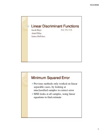
Linear Discriminant Analysis • If we have samples corresponding to two or more classes, we prefer to select those features that best discriminate between classes – rather than those that best describe the data. • This will, of course, depend on the classifier. • Assume our classifier is Bayes. • Thus, we want to minimize the probability of error. • We will develop a method based on scatter matrices. Theorem • Let the samples of two classes be Normally distributed in R p , with common covariance matrix. Then, the Bayes errors in the p -dimensional space and in the one-dimensional subspace given by v = S - 1 ( µ 1 - µ 2 )/|| S - 1 ( µ 1 - µ 2 ) ||, are the same; where || x || is the Euclidean norm of the vector x . • That is, there is no loss in classification when reducing from p dimensions to one . 1 n 1 m å å = = error l ( y , f ( x )) ; error l ( z , f ( t )) . training i i testing i i n n i = 1 i = 1 PCA LDA 1 n å = - T 2 error ( y v x v ) training i i n = i 1 2
LDA LDA Fisherfaces (LDA) 3
Scatter matrices and separability criteria • Within-class scatter matrix: ( )( ) . C N åå = - µ - µ T S x x W ij j ij j = = j 1 i 1 • Between-class scatter matrix: ( )( ) . C å T = µ - µ µ - µ S B j j = j 1 ˆ S = + • Note that: S S . W B • To formulate criteria for class separability, we need to convert these matrices to numerical values: - 1 tr ( S S ) 2 1 - ln | S | ln | S | 1 2 tr S 1 tr S 2 • Typical combination of scatter matrices are: ˆ ˆ = S S { S , S } { S , S }, { S , }, and { S , }. 1 2 B W B W A solution to LDA • Again, we want to minimize the Bayes error. • Therefore, we want the projection from Y to X that minimizes the error: p n å å ˆ = f + f X ( p ) y b . i i i i = = + i 1 i p 1 • The eigenvalue decomposition is the optimal ( ) transformation: - 1 f = l f S W S . B i i i Simultaneous diagonalization. 4
Ronald Fisher (1890-1962) • Fisher was an eminent scholar and one of the great scientist of the first part of the 20 th century. After graduating from Cambridge and being denied entry to the British army for his poor eyesight, he worked as a statistician for six years before starting a farming business. While a farmer, he continued his genetics and statistics research. During this time, he developed the well-known analysis of variance (ANOVA) method. After the war, Fisher finally moved to Rothamsted Experimental Station. Among his many accomplishments, Fisher invented ANOVA, the technique of maximum likelihood (ML), Fisher Information, the concept of sufficiency, and the method now known as Linear Discriminant Analysis(LDA). During World War II, the filed of eugenics suffered a big blow -- mainly do to the Nazis use of it as a justification for some of their actions. Fisher moved back to Rothamsted and then to Cambridge wherehe retired. Fisher has been accredited to be one of the founders of modern statistics and one cannot study pattern recognition without encountering several of his ground-breaking insights. Yet as great as a statistician that he was, he also become a major figure in genetics. A classical quote in the Annals of Statistics reads � I occasionally meet geneticists who ask me whether it is true that the great geneticist R.A. Fisher was also an important statistician." Example : Face Recognition 5
Limitations of LDA • To prevent to become singular, N>d . S W • There are only C-1 nonzero eigenvectors. • • Nonparametric LDA is design to solve the last problem (we � ll see this latter in the course). PCA versus LDA • In many applications the number of samples is relatively small compared to the dimensionality of the data. • Even for simple PDFs, PCA can outperform LDA (testing data). • Again, this limits the number of features one can use. • PCA is usually a guarantee, because all we try to do is to minimize the representation error. underlying but unknown PDFs 6
Problems with Multi-class Eigen-based Algorithms • In general, researchers define algorithms which are optimal in the 2-classes case and then extend this idea (way of thinking) to the multi-class problem. • This may caused problems. • This is the case for eigen-based approaches which use the idea of scatter matrices defined above. = L M V M V . • Let � s define the general case: 1 2 • This is the same as selecting those eigenvectors v that maximize: T v M v 1 T v M v 2 • Note that this can only be achieved if M 1 and M 2 agree. • The existence of solution depends on the angle between the eigenvectors of M 1 and M 2 . v i is the i th basis vector of the solution space. w i are the eigenvectors of M 1 . u i are the eigenvectors of M 2 . 7
How to know? ( ) ( ) r i r i åå åå 2 2 = q = T K cos u w . ij j i i = 1 j = 1 i = 1 j = 1 where r < q and q is the number of eigenvectors of M 1 . • The larger K is, the less probable that the results will be correct. 8
Recommend
More recommend
Explore More Topics
Stay informed with curated content and fresh updates.
