Introduction to Linear Quadratic Regulation Robert Platt Computer - PDF document
Introduction to Linear Quadratic Regulation Robert Platt Computer Science and Engineering SUNY at Buffalo February 13, 2013 1 Linear Systems A linear system has dynamics that can be represented as a linear equation. Let x t R n denote the
Introduction to Linear Quadratic Regulation Robert Platt Computer Science and Engineering SUNY at Buffalo February 13, 2013 1 Linear Systems A linear system has dynamics that can be represented as a linear equation. Let x t ∈ R n denote the state 1 of the system at time t . Let u t ∈ R m denote the action (also called the control ) taken by the system at time t . Linear system dynamics can always be represented in terms of an equation of the following form: x t +1 = Ax t + Bu t , (1) where A ∈ R n × n is a constant n × n matrix and B ∈ R n × m is a constant n × m matrix. Given that the system takes action u t from state x t , this equation allows us to predict the state of the next time step. The reason we call Equation 1 a linear equation is that is it linear in the variables, x t and u t . 2 Another thing to notice about the above equation is that it is written in terms of the states and actions taken at discrete time steps. As a result, we refer to this as a discrete time system. A classic example of a linear system is the damped mass. Imagine applying forces to an object lying on a frictional surface. Denote the mass of the object by m and the coefficient of friction r t ∈ R n denote the position, velocity, and acceleration of the object, r t ∈ R n , and ¨ by b . Let r t , ˙ respectively. There are three forces acting on the object. The inertial force at time t is m ¨ r t . The frictional (viscous friction) force is b ˙ r t . Let the applied force at time t be denoted f t . The motion of the object is described by the following second order differential equation known as the equation of motion : m ¨ r t + b ˙ r t = f t . 1 State is assumed to be Markov in the sense that it is a sufficient statistic to predict future system behavior. 2 If one of these variables were squared (for example, x t +1 = Ax 2 t + Bu t ), then this equation would no longer be linear. 1
Suppose we want to write the equation of motion of the object in as a discrete time equation of the form of Equation 1. Choose (arbitrarily) a period between successive time steps as 0 . 1 seconds. The position at time t + 1 is: r t +1 = r t + 0 . 1 ˙ r t . (2) The velocity at time t + 1 is: r t +1 ˙ = r t + 0 . 1¨ ˙ r t r t + 0 . 1 1 = ˙ m ( f t − b ˙ r t ) . (3) Then Equations 2 and 3 can be written as a system of two equations as follows: � r t +1 � 1 � � r t � 0 � � � 0 . 1 = + u t . 1 − 0 . 1 b r t +1 ˙ 0 r t ˙ 0 . 1 m This can be re-written as: x t +1 = Ax t + Bu t , where � r t � x t = , ˙ r t � 1 � 0 . 1 A = , 1 − 0 . 1 b 0 m and � 0 � B = . 0 . 1 2 Control Via Least Squares Consider an initial state, x 1 , and a sequence of T − 1 actions, u = ( u 1 , . . . , u T − 1 ) T . Using the system dynamics Equation 1, we can calculate the corresponding sequence of states. Let x = ( x 1 , . . . , x T ) T be the sequence of T states such that Equation 1 is satisfied (the trajectory of states visited by the system as a result of taking the action sequence, u ). The objective of control is to take actions that cause the following cost equation to be minimized: T − 1 � J ( x , u ) = x T x T t Qx t + u T T Q F x T + t Ru t , (4) t =1 where Q ∈ R n × n and Q F ∈ R n × n determine state costs and R ∈ R m × m determines action costs. 2
One way to solve the control problem for linear systems with quadratic cost functions is to solve a least squares problem. Suppose that the sequence of actions, u = ( u 1 , . . . , u T − 1 ) T , is taken starting in state x 1 at time t = 1 . The state at time t = 2 is: x 2 = Ax 1 + Bu 1 . The state of time t = 3 is: = A ( Ax 1 + Bu 1 ) + Bu 2 x 3 A 2 x 1 + ABu 1 + Bu 2 . = The state of time t = 4 is: A ( A 2 x 1 + ABu 1 + Bu 2 ) + Bu 3 x 4 = A 3 x 1 + A 2 Bu 1 + ABu 2 + Bu 3 . = The entire trajectory of states over time horizon T can be calculated in a similar way: 0 0 0 0 . . . 0 I 0 0 0 0 B . . . A AB B 0 0 . . . 0 A 2 A 2 B 0 0 AB B . . . = u + x 1 x A 3 A 3 B A 2 B AB B . . . 0 . . . . . . . . . A T A T − 1 B A T − 2 B A T − 3 B A T − 4 B . . . B = G u + Hx 1 . (5) The cost function can also be “vectorized”: 0 0 0 0 Q . . . R . . . 0 Q . . . 0 0 R . . . 0 x T x + u T J = . . . . u . . . . . . . . 0 0 . . . Q F 0 0 . . . R x T Q x + u T R u = ( G u + Hx 1 ) T Q ( G u + Hx 1 ) + u T R u = (6) (7) The control problem can be solved by finding a u that minimizes Equation 7. This is a least squares problem and can be solved using the pseudoinverse. For simplicity, assume that R is zero. 3 In this case, the objective is to find the u that minimizes the following L 2 norm: � Q 1 / 2 G u + Q 1 / 2 Hx 1 � 2 . 3 The case where R is non-zero can be solved by writing Equation 7 as a quadratic form by completing the square. 3
The least squares solution is: u = ( Q 1 / 2 G ) + Q 1 / 2 Hx 1 , (8) where ( · ) + denotes the pseudoinverse 4 3 Control Via Dynamic Programming Equation 8 calculates an optimal control, u , in the sense that no other control will achieve a lower cost, J . However, it can be inconvenient to use the direct least squares method to calculate control because of the need to create those big matrices. Moreover, the solution requires inverting a big matrix. In this section, I introduce an alternative method for calculating the same solution that uses the Bellman optimality equation 5 . Let V t ( x ) denote the optimal value function at x at time t . Specifically, V t ( x ) is equal to the future cost that would be experienced by the system if the optimal policy is followed. This is similar to the way we defined the value function in Reinforcement Learning (RL). However, whereas the value function in the RL section denoted expected future rewards, the value function in this discussion denotes future costs. The Bellman equation 6 is: x T Qx + u T Ru + V t +1 ( Ax + bu ) � � V t ( x ) = min . (9) u ∈ R m Assume that we somehow know 7 that the value function at time t + 1 is a quadratic of the form, V t +1 ( x ) = x T P t +1 x, (10) where P t +1 is a positive semi-definite matrix 8 . In this case, the Bellman equation becomes: V t ( x ) = x T Qx min u T Ru + ( Ax + bu ) T P t +1 ( Ax + bu ) � � . (11) u ∈ R m In the above, we are minimizing a quadratic function. As a result, we can calculate the global minimum by setting the derivative to zero: ∂ u T Ru + ( Ax + bu ) T P t +1 ( Ax + bu ) � � 0 = ∂u 2 u T R + 2 x T A T P t +1 B + u T B T P t +1 B. = 4 Recall that for a non-singular matrix A , A + = ( A T A ) − 1 A T when A is tall (rows greater than columns) and A + = A T ( AA T ) − 1 when A is fat (columns greater than rows). 5 The same bellman optimality equation we studied in the section on Reinforcement Learning. 6 Often called the Hamilton-Jacobi-Bellman equation in the controls literature. 7 Leprechauns told us? 8 A matrix is positive semi-definite if all its eigenvalues are non-negative. 4
Recommend
More recommend
Explore More Topics
Stay informed with curated content and fresh updates.
