11. Quadratic forms and ellipsoids Quadratic forms Orthogonal - PowerPoint PPT Presentation
CS/ECE/ISyE 524 Introduction to Optimization Spring 201718 11. Quadratic forms and ellipsoids Quadratic forms Orthogonal decomposition Positive definite matrices Ellipsoids Laurent Lessard (www.laurentlessard.com) Quadratic
CS/ECE/ISyE 524 Introduction to Optimization Spring 2017–18 11. Quadratic forms and ellipsoids ❼ Quadratic forms ❼ Orthogonal decomposition ❼ Positive definite matrices ❼ Ellipsoids Laurent Lessard (www.laurentlessard.com)
Quadratic forms ❼ Linear functions: sum of terms of the form c i x i where the c i are parameters and x i are variables. General form: c 1 x 1 + · · · + c n x n = c T x ❼ Quadratic functions: sum of terms of the form q ij x i x j where q ij are parameters and x i are variables. General form: ( n 2 terms) q 11 x 2 1 + q 12 x 1 x 2 + · · · + q nn x 2 n T x 1 q 11 . . . q 1 n x 1 . . . . ... = x T Qx . . . . = . . . . x n q n 1 q nn x n . . . 11-2
Quadratic forms Example: 4 x 2 + 6 xy − 2 yz + y 2 − z 2 T x 4 6 0 x 0 1 0 y y z 0 − 2 − 1 z T x 4 p 2 q 2 x p 1 + p 2 = 6 In general: 1 q 1 + q 2 = 0 y p 1 r 2 y z q 1 r 1 − 1 z r 1 + r 2 = − 2 T x 4 3 0 x Symmetric: y 3 1 − 1 y 0 − 1 − 1 z z 11-3
Quadratic forms Any quadratic function f ( x 1 , . . . , x n ) can be written in the form x T Qx where Q is a symmetric matrix ( Q = Q T ). Proof: Suppose f ( x 1 , . . . , x n ) = x T Rx where R is not symmetric. Since it is a scalar, we can take the transpose: � T = x T R T x x T Rx = � x T Rx Therefore: x T Rx = 1 � x T Rx + x T R T x � = x T 1 2 ( R + R T ) x 2 So we’re done, because 1 2 ( R + R T ) is symmetric! 11-4
Orthogonal decomposition Theorem . Every real symmetric matrix Q = Q T ∈ R n × n can be decomposed into a product: Q = U Λ U T where Λ = diag( λ 1 , . . . , λ n ) is a real diagonal matrix, and U ∈ R n × n is an orthogonal matrix. i.e. it satisfies U T U = I . This is a useful decomposition because orthogonal matrices have very nice properties... 11-5
Orthogonal matrices A matrix U is orthogonal if U T U = I . � � ❼ If the columns are U = · · · , then we have: u 1 u 2 u m u T u T 1 u 1 · · · 1 u m 1 · · · 0 . . . . ... ... U T U = . . . . = . . . . u T u T · · · 0 · · · 1 m u 1 m u m Columns of U are mutually orthogonal: u T i u j = 0 if i � = j . ❼ If U is square, U − 1 = U T , and U T is also orthogonal. 11-6
Orthogonal matrices ❼ columns can be rearranged and the factorization stays valid. u T 0 0 λ 1 1 u T � � u 1 u 2 u 3 0 λ 2 0 2 u T 0 0 λ 3 3 = λ 1 u 1 u T 1 + λ 2 u 2 u T 2 + λ 3 u 3 u T 3 u T λ 1 0 0 1 � � u T = u 1 u 3 u 2 0 0 λ 3 3 u T 0 0 λ 2 2 11-7
Orthogonal matrices ❼ Orthogonal matrices preserve angle and (2-norm) distance: ( Ux ) T ( Uy ) = x T ( U T U ) y = x T y In particular, we have � Uz � = � z � for any z . ❼ If Q = U Λ U T , then multiply by u i : T u T u T λ 1 · · · 0 1 1 . . . . ... . . . . Qu i = u i = λ i u i . . . . u T u T 0 · · · λ n n n So multiplication by Q simply scales each u i by λ i . In other words: ( λ i , u i ) are the eigenvalue-eigenvector pairs of Q . 11-8
Orthogonal matrix example Rotation matrices are orthgonal: � cos θ � sin θ R θ = − sin θ cos θ We can verify this: � � cos θ � cos θ � − sin θ sin θ R T θ R θ = sin θ cos θ − sin θ cos θ cos 2 θ + sin 2 θ � � cos θ sin θ − sin θ cos θ = sin 2 θ + cos 2 θ sin θ cos θ − cos θ sin θ � 1 � 0 = 0 1 Note: R T θ = R − θ . This holds for 3 D rotation matrices also... 11-9
Eigenvalues and eigenvectors If A ∈ R n × n and there is a vector v and scalar λ such that Av = λ v Then v is an eigenvector of A and λ is the corresponding eigenvalue . Some facts: ❼ Any square matrix has n eigenvalues. ❼ Each eigenvalue has at least one corresponding eigenvector. ❼ In general, eigenvalues & eigenvectors can be complex. ❼ In general, eigenvectors aren’t orthogonal, and may not � � even be linearly independent. i.e. V = v 1 · · · v n may not be invertible. If it is, we say that A is diagonalizable and then A = V Λ V − 1 . Otherwise, Jordan Canonical Form. ❼ Symmetric matrices are much simpler! 11-10
Recap: symmetric matrices ❼ Every symmetric Q = Q T ∈ R n × n has n real eigenvalues λ i . ❼ There exist n mutually orthogonal eigenvectors u 1 , . . . , u n : Qu i = λ i u i for all i = 1 , . . . , n � 1 if i = j u T i u j = 0 if i � = j � � then U T U = I and ❼ If we define U = · · · u 1 u n λ 1 · · · 0 . . ... . . U T Q = U . . 0 · · · λ n 11-11
Eigenvalue example Consider the quadratic: 7 x 2 + 4 xy + 6 y 2 + 4 yz + 5 z 2 . A simple question: are there values that make this negative? T 7 2 0 x x equivalent to: y 2 6 2 y 0 2 5 z z Orthogonal decomposition: T − 1 2 2 − 1 2 2 3 0 0 7 2 0 3 3 3 3 3 3 = 2 − 1 2 2 − 1 2 2 6 2 0 6 0 3 3 3 3 3 3 0 2 5 − 2 − 2 1 − 2 − 2 1 0 0 9 3 3 3 3 3 3 Eigenvalues are { 3 , 6 , 9 } . 11-12
Eigenvalue example Eigenvalue decomposition: T − 1 2 2 − 1 2 2 3 0 0 7 2 0 3 3 3 3 3 3 = 2 − 1 2 2 − 1 2 2 6 2 0 6 0 3 3 3 3 3 3 0 2 5 − 2 − 2 1 − 2 − 2 1 0 0 9 3 3 3 3 3 3 Define new coordinates: T − 1 2 2 p x 3 3 3 = 2 − 1 2 q y 3 3 3 r z − 2 − 2 1 3 3 3 Then we can write: T T 7 2 0 3 0 0 x x p p = y 2 6 2 y q 0 6 0 q z 0 2 5 z r 0 0 9 r 11-13
Eigenvalue example After some manipulations, we discovered that 7 x 2 + 4 xy + 6 y 2 + 4 yz + 5 z 2 = 3 p 2 + 6 q 2 + 9 r 2 where: − 1 3 x + 2 3 y − 2 p = 3 z 3 x − 1 2 3 y − 2 q = 3 z 2 3 x + 2 3 y + 1 r = 3 z Conclusion: the quadratic can never be negative. 11-14
Recap Question: Is x T Qx ever negative? Answer: Look at the orthogonal decomposition of Q : ❼ Q = U Λ U T ❼ Define new coordinates z = U T x . ❼ x T Qx = λ 1 z 2 1 + · · · + λ n z 2 n If all λ i ≥ 0, then x T Qx ≥ 0 for any x . If some λ k < 0, set z k = 1 and all other z i = 0. Then find corresponding x using x = Uz , and x T Qx < 0. 11-15
Positive definite matrices For a matrix Q = Q T , the following are equivalent: 1. x T Qx ≥ 0 for all x ∈ R n 2. all eigenvalues of Q satisfy λ i ≥ 0 A matrix with this property is called positive semidefinite (PSD). The notation is Q � 0. Note: When we talk about PSD matrices, we always assume we’re talking about a symmetric matrix. 11-16
Positive definite matrices Name Definition Notation Positive semidefinite all λ i ≥ 0 Q � 0 Positive definite all λ i > 0 Q ≻ 0 Negative semidefinite all λ i ≤ 0 Q � 0 Negative definite all λ i < 0 Q ≺ 0 Indefinite everything else (none) Some properties: ❼ If P � 0 then − P � 0 ❼ If P � 0 and α > 0 then α P � 0 ❼ If P � 0 and Q � 0 then P + Q � 0 ❼ Every R = R T can be written as R = P − Q for some appropriate choice of matrices P � 0 and Q � 0. 11-17
Ellipsoids ❼ For linear constraints, the set of x satisfying c T x = b is a hyperplane and the set c T x ≤ b is a halfspace . ❼ For quadratic constraints: If Q ≻ 0, the set x T Qx ≤ b is an ellipsoid . 11-18
Ellipsoids ❼ By orthogonal decomposition, we can write x T Qx = z T Λ z where we defined the new coordinates z = U T x . ❼ The set of x satisfying x T Qx ≤ 1 corresponds to the set of z satisfying λ 1 z 2 1 + · · · + λ n z 2 n ≤ 1. ❼ If Q ≻ 0, then λ i > 0. In the z coordinates, this is a stretched sphere (ellipsoid). In the z i direction, it is 1 stretched by √ λ i . ❼ Since x = Uz , and this transformation preserves angles and distances (think of it as a rotation), then in the x i coordinates, it is a rotated ellipsoid. ❼ The principal axes (the z i directions) map to the u i directions after the rotation. 11-19
Ellipsoids Plot of the region 3 p 2 + 6 q 2 + 9 r 2 ≤ 1 Ellipse axes are in the directions e 1 , e 2 , e 3 Plot of the region 7 x 2 + 4 xy + 6 y 2 + 4 yz + 5 z 2 ≤ 1 Ellipse axes are in the directions u 1 , u 2 , u 3 11-20
Norm representation If Q � 0 we can define the matrix square root : 1. Let Q = U Λ U T be an orthogonal decomposition 2. Let Λ 1 / 2 = diag( √ λ 1 , . . . , √ λ n ) 3. Define Q 1 / 2 = U Λ 1 / 2 U T . We have the property that Q 1 / 2 is symmetric and Q 1 / 2 Q 1 / 2 = Q . Also: � 2 x T Qx = ( Q 1 / 2 x ) T ( Q 1 / 2 x ) = � � Q 1 / 2 x � � 2 ≤ b Therefore: x T Qx ≤ b � � Q 1 / 2 x � ⇐ ⇒ 11-21
Recommend
More recommend
Explore More Topics
Stay informed with curated content and fresh updates.
