1. The General Linear-Quadratic Framework Notation: x = ( x j ) , - PowerPoint PPT Presentation
ECO 317 Economics of Uncertainty Fall Term 2009 Slides to accompany 21. Incentives for Effort - Multi-Dimensional Cases 1. The General Linear-Quadratic Framework Notation: x = ( x j ) , n -vector of agents effort (tasks), private
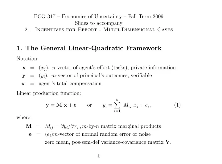
ECO 317 – Economics of Uncertainty – Fall Term 2009 Slides to accompany 21. Incentives for Effort - Multi-Dimensional Cases 1. The General Linear-Quadratic Framework Notation: x = ( x j ) , n -vector of agent’s effort (tasks), private information = ( y i ) , m -vector of principal’s outcomes, verifiable y w = agent’s total compensation Linear production function: n � y = M x + e or y i = M ij x j + e i , (1) i =1 where M = M ij = ∂y i /∂x j , m -by- n matrix marginal products = ( e i ) m -vector of normal random error or noise e zero mean, pos-sem-def variance-covariance matrix V . 1
Linear compensation function: w = h + s ′ y (2) where h = fixed component = m -vector of marginal incentive bonus coefficients s Agent’s objective (utility, or payoff): 2 x ′ K x U A = E[ w ] − 1 2 α Var[ w ] − 1 (3) where α = agent’s coefficient of constant absolute risk aversion = n -by- n symmetric pos semi-def matrix K Two tasks i and j are substitutes if K ij > 0 (increase in x i raises marginal disutility of x j and vice versa), and complements if K ij < 0. Agent’s outside opportunity utility U 0 A . 2
Principal’s objective (utility, or payoff): U P = E[ p ′ y − w ] (4) where p is m -vector of unit valuations. 2. One Principal, One Agent We have w = h + s ′ y = h + s ′ M x + s ′ e Therefore E[ w ] = h + s ′ M x , Var[ w ] = s ′ V s and U A = h + s ′ M x − 1 2 α s ′ V s − 1 2 x ′ K x (5) The agent chooses x to maximize this. The vector FOC (MAT203) M ′ s − K x = 0 . (6) SOC: − K negative semi-definite, which is true. 3
FOC using MAT 201 methods: m n m m n n � � s i M ij x j − 1 � � s i V ik s k − 1 � � U A = h + x h K hj x j . 2 2 i =1 j =1 i =1 j =1 k =1 h =1 For any one component of x , say x g , we have m n n ∂U A � s i M ig − 1 � x h K hg − 1 � = K gj x j . ∂x g 2 2 i =1 h =1 j =1 Rearranging and collecting terms into vector and matrices yields (6). In the process, the matrices M and K have to be transposed, and you need to remember that the latter is symmetric. Solving (6) for x : x = K − 1 M ′ s Agent’s IC (7) E[ y ] = M K − 1 M ′ s ≡ N s , where M K − 1 M ′ m -by- m matrix of marginal products = N of bonus coefficients on principal’s outcomes 4
Agent’s maximized or indirect utility function: h + s ′ M [ K − 1 M ′ s ] − 1 2 α s ′ V s − 1 2 [ K − 1 M ′ s ] ′ K [ K − 1 M ′ s ] U ∗ = A 2 s ′ M K − 1 M ′ s − 1 2 α s ′ V s h + 1 = 2 s ′ N s − 1 2 α s ′ V s h + 1 = (8) Principal’s indirect utility function p ′ E[ y ] − E[ w ] U P = p ′ N s − h − s ′ M [ K − 1 M ′ s ] = p ′ N s − h − s ′ N s . = (9) A = U 0 Use agent’s binding PC U ∗ A to solve for h . Then p ′ N s − U 0 2 s ′ N s − 1 2 α s ′ V s − s ′ N s A + 1 U P = p ′ N s − U 0 2 s ′ N s − 1 2 α s ′ V s A − 1 = (10) Maximize this w.r.t. s , FOC is N p − [ N + α V ] s = 0 . (11) 5
SOC: ( N + α V ) positive semi-definite, which is true. Solving s = [ N + α V ] − 1 N p . (12) Check 1-dimensional special case: p = 1, M = 1, K = k , and V = v . Then N = 1 /k , and (12) becomes 1 s = [(1 /k ) + α v ] − 1 (1 /k ) = 1 + α v k . 6
3. One Task, Two Outcome Measures m = 2 and n = 1. Make M (now a 2-by-1 column vector) = (1 , 1) ′ by choice of units. Let the matrix V be diagonal, � 1 � � � � � = 1 v 1 0 1 1 1 � � V = ; then N = 1 1 , 0 v 2 1 1 1 k k and � � N + α V = 1 1 + k α v 1 1 . 1 1 + k α v 2 k Therefore � − 1 1 � � � 1 + k α v 1 1 1 1 s = k p . 1 1 + k α v 2 1 1 k This simplifies to v 2 ( p 1 + p 2 ) v 1 ( p 1 + p 2 ) s 1 = , s 2 = . v 1 + v 2 + k α v 1 v 2 v 1 + v 2 + k α v 1 v 2 7
Implications: [1] Even if p 2 = 0, s 2 � = 0. Depends only on ( p 1 + p 2 ). Outcome 2 is useful because of its information content. Observe s 1 /s 2 = v 2 /v 1 . If v 1 is large, rely on s 2 . [2]Even if α = 0, each of s 1 and s 2 is < ( p 1 + p 2 ). Specifically, s 1 = v 2 ( p 1 + p 2 ) s 2 = v 1 ( p 1 + p 2 ) , . v 1 + v 2 v 1 + v 2 Thus s 1 + s 2 = p 1 + p 2 . Total incentive has full power, but its split optimizes information. 8
4. Many tasks, Two Outcomes Dimension n of x can be large. Dimension m of outcomes = 2. Take p 2 = 0 so outcome 2 has only information role. Suppose constraint s 1 = 0 so compensation must be based on outcome 2. How useful is it? Take α = 0 to remove the issue of the agent’s risk aversion. Also assume K diagonal, k I n , to remove issue of effort interaction. � � � � � � � � N 11 N 12 0 N 11 N 12 0 − 1 U P = ( p 1 0 ) 2 ( 0 s 2 ) N 21 N 22 s 2 N 21 N 22 s 2 2 N 22 ( s 2 ) 2 . p 1 N 12 s 2 − 1 = The first-order condition (11) for s 2 (the only relevant component of s ) becomes N 22 s 2 = N 12 p 1 . Also N = M ( k I n ) − 1 M ′ = 1 k M M ′ . 9
Therefore n n N 22 = 1 N 12 = 1 ( M 2 j ) 2 , � � M 1 j M 2 j , k k j =1 j =1 and then n � M 1 j M 2 j j =1 s 2 = p 1 . n � ( M 2 j ) 2 j =1 The sign and magnitude of s 2 depend importantly on those of the nu- merator. This is inner product or covariance between the marginal effects of the actions on the two dimensions of outcome. (A large nega- tive alignment would be just as valuable as a large positive alignment, making s 2 big and negative. Zero alignment makes indicator 2 useless.) 10
5. Substitutes and Complements in Efforts Focus on effect of non-zero off-diagonal entries in K . Get rid of all else: [1] m = n = 2, [2] p 1 = p 2 = p , [3] M diagonal = I 2 by choice of units. [4] V also diagonal = v I 2 , [5] the disutility matrix is � � k θ k K = . θ k k where k > 0 and − 1 < θ < 1. Actions substitutes if θ > 0, complements if θ < 0. Then x = K − 1 I 2 s = K − 1 s , 11
so � − 1 � � � � � x 1 k θ k s 1 = x 2 θ k k s 2 � − 1 � � � 1 1 θ s 1 = θ 1 s 2 k � � � � 1 1 − θ s 1 = − θ 1 s 2 k (1 − θ 2 ) � � 1 s 1 − θ s 2 = (13) s 2 − θ s 1 k (1 − θ 2 ) This is another view of the substitutes / complements distinction. The two are equivalent in the 2-by-2 case but can differ in higher dimensions. 12
Now N = I 2 K − 1 I 2 = K − 1 , so FOC (11) becomes [ K − 1 + α v I 2 ] s = K − 1 p . Premultiplying by K gives [ I 2 + α v K ] s = p , or � � � � � � 1 + α v k θ α v k s 1 p = . θ α v k 1 + α v k s 2 p This yields the solution p s 1 = s 2 = 1 + (1 + θ ) α v k . Substitutes ( θ > 0), make it necessary to reduce the power of incen- tives on both outcomes, because sharpening the incentives on either will cause the agent to divert his effort away from the other. Conversely, complements ( θ < 0) enable strengthening of incentives to both tasks. Implications for organization theory: when grouping tasks into de- partments, group together complements. Think of universities, IRS, Homeland Security etc. in this perspective. 13
6. Multiple Principals – Common Agency Two actions and two outcomes ( m = n = 2). Production function M = I 2 ; so each action affects only one outcome. Disutility of effort K = k I 2 , so no substitutes/complement issue. 1 k I 2 I 2 = 1 N = I 2 k I 2 Error variance matrix V = v I 2 . Two principals. Each cares about only one outcome. If they jointly implement the incentive scheme, p 1 p 2 s 1 = 1 + α v k, s 2 = (14) 1 + α v k We want non-cooperative Nash equilibrium of principals’ individual choices. So now let the two principals act independently, offer respectively w 1 = h 1 + s 1 , 1 y 1 + s 1 , 2 y 2 (15) w 2 = h 2 + s 2 , 1 y 1 + s 2 , 2 y 2 (16) Note: each includes the other’s outcome to affect the agent’s action. 14
Agent’s total compensation w = h + s 1 y 1 + s 2 y 2 where h = h 1 + h 2 , s 1 = s 1 , 1 + s 2 , 1 , s 2 = s 1 , 2 + s 2 , 2 Then, from (7) the agent’s effort choice is given by � � � � � � � � x 1 1 /k 0 1 0 s 1 = x 2 0 1 /k 0 1 s 2 or x = s / k or x 1 = s 1 k = s 1 , 1 + s 2 , 1 x 2 = s 2 k = s 1 , 2 + s 2 , 2 , k k 15
Then E[ w 1 ] = h 1 + s 1 , 1 x 1 + s 1 , 2 x 2 s 1 s 2 = h 1 + s 1 , 1 k + s 1 , 2 k h 1 + 1 = k [ s 1 , 1 ( s 1 , 1 + s 2 , 1 ) + s 1 , 2 ( s 1 , 2 + s 2 , 2 ) ] Using the special forms of N and V , h + 1 2 k s ′ s − 1 2 α v s ′ s U ∗ = A � 1 2 k − α v � � ( s 1 , 1 + s 2 , 1 ) 2 + ( s 1 , 2 + s 2 , 2 ) 2 � = h 1 + h 2 + (17) 2 16
Focus on principal 1. s 1 , 1 + s 2 , 1 − h 1 − 1 U 1 P = E[ p 1 y 1 − w 1 ] = p 1 k [ s 1 , 1 ( s 1 , 1 + s 2 , 1 ) + s 1 , 2 ( s 1 , 2 + s 2 , 2 ) ] k He chooses ( h 1 , s 1 , 1 , s 1 , 2 ) to max this, given principal 2’s ( h 2 , s 2 , 1 , s 2 , 2 ) A ≥ U 0 and respecting the agent’s participation constraint U ∗ A . So � 1 2 k − α v � � ( s 1 , 1 + s 2 , 1 ) 2 + ( s 1 , 2 + s 2 , 2 ) 2 � h 1 = U 0 A − h 2 − 2 and � 1 s 1 , 1 + s 2 , 1 2 k − α v � � ( s 1 , 1 + s 2 , 1 ) 2 + ( s 1 , 2 + s 2 , 2 ) 2 � U 1 − U 0 = p 1 A + h 2 + P k 2 − 1 k [ s 1 , 1 ( s 1 , 1 + s 2 , 1 ) + s 1 , 2 ( s 1 , 2 + s 2 , 2 ) ] 17
Recommend
More recommend
Explore More Topics
Stay informed with curated content and fresh updates.
