Algorithms (2IL15) Lecture 12 Linear Programming 1 TU/e - PowerPoint PPT Presentation
TU/e Algorithms (2IL15) Lecture 12 Algorithms (2IL15) Lecture 12 Linear Programming 1 TU/e Algorithms (2IL15) Lecture 12 Summary of previous lecture -approximation algorithm: algorithm for which computed solution is within
TU/e Algorithms (2IL15) – Lecture 12 Algorithms (2IL15) – Lecture 12 Linear Programming 1
TU/e Algorithms (2IL15) – Lecture 12 Summary of previous lecture ρ -approximation algorithm: algorithm for which computed solution is within factor ρ from OPT to prove approximation ratio we usually need lower bound on OPT (or, for maximization, upper bound) PTAS = polynomial-time approximation scheme = algorithm with two parameters, input instance and ε > 0, such that approximation ratio is1+ ε – running time is polynomial in n for constant ε – FPTAS = PTAS whose running time is polynomial in 1/ ε some problems are even hard to approximate 2
TU/e Algorithms (2IL15) – Lecture 12 Today: linear programming (LP) most used and most widely studied optimization method can be solved in polynomial time (input size measured in bits) can be used to model many problems also used in many approximation algorithms (integer LP + rounding) we will only have a very brief look at LP … what is LP? what are integer LP and 0/1-LP ? how can we model problems as an LP ? … and not study algorithms to solve LP’s 3
TU/e Algorithms (2IL15) – Lecture 12 Example problem: running a chocolate factory Assortment caca mil hazelnut retail price (100 o k s g) Pure Black 1 0 0 1.99 Creamy Milk 0.6 0.4 0 1.49 Hazelnut 0.6 0.2 0.2 1.69 Delight Super Nuts 0.5 0.1 0.4 1.79 Cost and availability of ingredients cost (kg) available (kg) How much should we produce of each product to maximize our profit ? cacao 2.1 50 milk 0.35 50 hazelnuts 1.9 30 4
TU/e Algorithms (2IL15) – Lecture 12 Modeling the chocolate-factory problem cacao milk hazelnuts price (100 g) Pure Black 1 0 0 1.99 cost (kg) available (kg) Creamy Milk 0.6 0.4 0 1.49 cacao 2.1 50 Hazelnut Delight 0.6 0.2 0.2 1.69 milk 0.35 50 Super Nuts 0.5 0.1 0.4 1.79 hazelnuts 1.9 30 variables we want to determine: production (kg) of the products b = production of Pure Black m = production of Creamy Milk h = production of Hazelnut Delight s = production of Super Nuts 5
TU/e Algorithms (2IL15) – Lecture 12 Modeling the chocolate-factory problem (cont’d) cacao milk hazelnuts price (100 g) Pure Black 1 0 0 1.99 cost (kg) available (kg) Creamy Milk 0.6 0.4 0 1.49 cacao 2.1 50 Hazelnut Delight 0.6 0.2 0.2 1.69 milk 0.35 50 Super Nuts 0.5 0.1 0.4 1.79 hazelnuts 1.9 30 profits (per kg) of the products Pure Black 19.9 – 2.1 = 17.8 Creamy Milk 14.9 – 0.6 x 2.1 + 0.4 x 0.35 = 13.5 Hazelnut Delight 15.19 Super Nuts: 16.055 total profit: 17.8 b + 13.5 m + 15.19 h + 16.055 s 6
TU/e Algorithms (2IL15) – Lecture 12 Modeling the chocolate-factory problem cacao milk hazelnuts price (100 g) Pure Black 1 0 0 1.99 cost (kg) available (kg) Creamy Milk 0.6 0.4 0 1.49 cacao 2.1 50 Hazelnut Delight 0.6 0.2 0.2 1.69 milk 0.35 50 Super Nuts 0.5 0.1 0.4 1.79 hazelnuts 1.9 30 we want to maximize the total profit 17.8 b + 13.5 m + 15.19 h + 16.055 s under the constraints b + 0.6 m + 0.6 h + 0.5 s ≤ 50 (cacao availability) 0.4 m + 0.2 h + 0.1 s ≤ 50 (milk availability) 0.2 h + 0.4 s ≤ 30 (hazelnut availability) This is a linear program: optimize linear function, under set of linear constraints 7
TU/e Algorithms (2IL15) – Lecture 12 Linear programming n variables; here n=2 , in chocolate example n=4, but often n is large Find values of real variables x, y such that y y ≤ ½ x + 2 x − 3 y is maximized subject to the constraints 1 − 2 x + y ≥ − 4 −3 x + y ≥ 3 − ½ x + y ≤ 2 y ≥ 0 x y ≥ 0 y ≥ 2x − 4 y ≥ − x + 3 m constraints: objective function; must be linear function ≤ constant linear function in the variables goal: maximize (or minimize) or ≥ or =, > and < not allowed 8
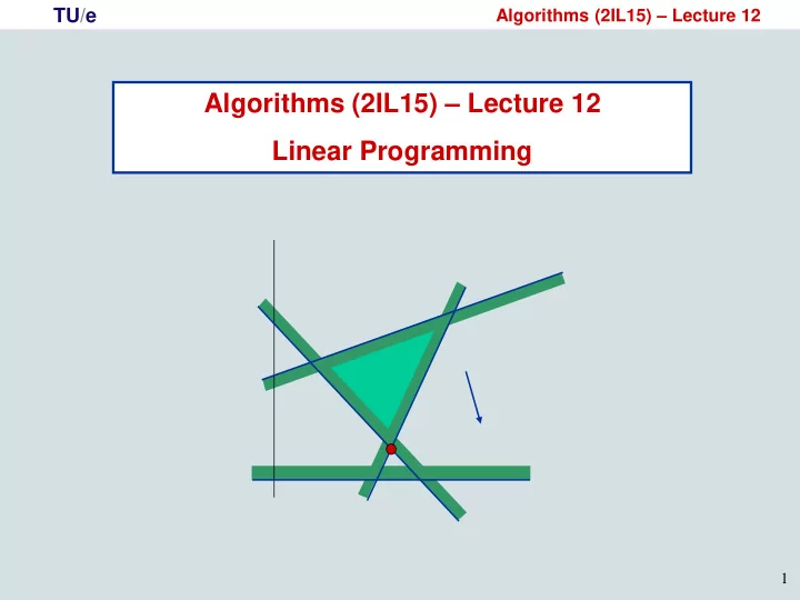
TU/e Algorithms (2IL15) – Lecture 12 Linear programming Find values of real variables x, y such that y = ½ x + 2 x − 3 y is maximized subject to the constraints 1 − 2 x + y ≥ − 4 −3 x + y ≥ 3 − ½ x + y ≤ 2 y = 0 y ≥ 0 y = 2x − 4 y = − x + 3 feasible region = region containing feasible solutions = region containing solutions satisfying all constraints feasible region is convex polytope in n -dim space 9
TU/e Algorithms (2IL15) – Lecture 12 Linear programming: Find values of real variables x 1 , …, x n such that given linear function c 1 x 1 + c 2 x 2 + … + c n x n is maximized (or: minimized) and given linear constraints on the variables are satisfied constraints: equalities or inequalities using ≥ or ≤, cannot use < and > Possible outcomes: unique optimal solution: vertex of feasible region 10
TU/e Algorithms (2IL15) – Lecture 12 Linear programming: Find values of real variables x 1 , …, x n such that given linear function c 1 x 1 + c 2 x 2 + … + c n x n is maximized (or: minimized) and given linear constraints on the variables are satisfied constraints: equalities or inequalities using ≥ or ≤, cannot use < and > Possible outcomes: unique optimal solution: vertex of feasible region no solution: feasible region in empty 11
TU/e Algorithms (2IL15) – Lecture 12 Linear programming: Find values of real variables x 1 , …, x n such that given linear function c 1 x 1 + c 2 x 2 + … + c n x n is maximized (or: minimized) and given linear constraints on the variables are satisfied constraints: equalities or inequalities using ≥ or ≤, cannot use < and > Possible outcomes: no solution: feasible region in empty unique optimal solution: vertex of feasible region bounded optimal solution, but not unique 12
TU/e Algorithms (2IL15) – Lecture 12 Linear programming: Find values of real variables x 1 , …, x n such that given linear function c 1 x 1 + c 2 x 2 + … + c n x n is maximized (or: minimized) and given linear constraints on the variables are satisfied constraints: equalities or inequalities using ≥ or ≤, cannot use < and > Possible outcomes: no solution: feasible region in empty unique optimal solution: vertex of feasible region bounded optimal solution, but not unique unbounded optimal solution 13
TU/e Algorithms (2IL15) – Lecture 12 Linear programming: standard form Maximize c 1 x 1 + c 2 x 2 + … + c n x n only “≤” a 1,1 x 1 + a 1,2 x 2 + … + a 1,n x n ≤ b 1 Subject to (no “=“ and no “≥”) a 2,1 x 1 + a 2,2 x 2 + … + a 2,n x n ≤ b 2 . ... a m,1 x 1 + a m,2 x 2 + … + a m,n x n ≤ b m not: minimize x 1 ≥ 0 x 2 ≥ 0 non-negativity constraints … for each variable x n ≥ 0 m x n matrix Maximize c∙x subject to A x ≤ b and non-negativity constraints on all x i n -dimensional vectors c, A, b are input, x must be computed 14
TU/e Algorithms (2IL15) – Lecture 12 Lemma: Any LP with n variables and m constraints can be rewritten as an equivalent LP in standard form with 2n variables and 2n+2m constraints. Proof. LP may not be in standard form because minimization instead of maximization − negate objective function: minimize 2 x 1 − x 2 + 4 x 3 maximize − 2 x 1 + x 2 − 4 x n some constraints are ≥ or = instead of ≤ − getting rid of =: replace 3 x + x 2 − x 3 = 5 3 x + x 2 − x 3 ≤ 5 by 3 x + x 2 − x 3 ≥ 5 − changing ≥ to ≤: negate constraint 3 x + x 2 − x 3 ≥ 5 − 3 x − x 2 + x 3 ≤ − 5 15
TU/e Algorithms (2IL15) – Lecture 12 Lemma: Any LP with n variables and m constraints can be rewritten as an equivalent LP in standard form with 2n variables and 2n+2m constraints. Proof (cont’d). LP may not be in standard form because minimization instead of maximization some constraints are ≥ or = instead of ≤ variables without non-negativity constraint − for each such variable x i introduce two new variables u i and v i − replace each occurrence of x i by ( u i − v i ) − add non-negativity constraints u i ≥ 0 and v i ≥ 0 16
TU/e Algorithms (2IL15) – Lecture 12 Lemma: Any LP with n variables and m constraints can be rewritten as an equivalent LP in standard form with 2n variables and 2n+2m constraints. Proof (cont’d). variables without non-negativity constraint − for each such variable x i introduce two new variables u i and v i − replace each occurrence of x i by ( u i − v i ) − add non-negativity constraints u i ≥ 0 and v i ≥ 0 new problem is equivalent to original problem : for any original solution there is new solution with same value − if x i ≥ 0 then u i = x i and v i = 0, otherwise u i = 0 and v i = − x i and vice versa − set x i = ( u i − v i ) 17
TU/e Algorithms (2IL15) – Lecture 12 Lemma: Any LP with n variables and m constraints can be rewritten as an equivalent LP in standard form with 2n variables and 2n+2m constraints. Instead of standard form, we can also get so-called slack form: – non-negativity constraint for each variable – all other constraints are =, not ≥ or ≤ Standard form (or slack form): convenient for developing LP algorithms When modeling a problem: just use general form 18
Recommend
More recommend
Explore More Topics
Stay informed with curated content and fresh updates.
