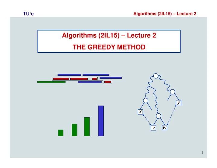
Algorithms (2IL15) Lecture 2 THE GREEDY METHOD y x w v 1 TU/e - PowerPoint PPT Presentation

TU/e Algorithms (2IL15) – Lecture 2 Algorithms (2IL15) – Lecture 2 THE GREEDY METHOD y x w v 1

TU/e Algorithms (2IL15) – Lecture 2 Optimization problems for each instance there are (possibly) multiple valid solutions   goal is to find an optimal solution • minimization problem: associate cost to every solution, find min-cost solution • maximization problem: associate profit to every solution, find max-profit solution 2

TU/e Algorithms (2IL15) – Lecture 2 Techniques for optimization optimization problems typically involve making choices backtracking: just try all solutions  can be applied to almost all problems, but gives very slow algorithms  try all options for first choice, for each option, recursively make other choices greedy algorithms: construct solution iteratively, always make choice that seems best  can be applied to few problems, but gives fast algorithms  only try option that seems best for first choice (greedy choice), recursively make other choices dynamic programming  in between: not as fast as greedy, but works for more problems 3

TU/e Algorithms (2IL15) – Lecture 2 Algorithms for optimization: how to improve on backtracking for greedy algorithms 1. try to discover structure of optimal solutions: what properties do optimal solutions have ?  what are the choices that need to be made ? do we have optimal substructure ?  optimal solution = first choice + optimal solution for subproblem  do we have greedy-choice property for the first choice ? 2. prove that optimal solutions indeed have these properties  prove optimal substructure and greedy-choice property 3. use these properties to design an algorithm and prove correctness  proof by induction (possible because optimal substructure) 4

TU/e Algorithms (2IL15) – Lecture 2 Today: two examples of greedy algorithms  Activity-Selection 8:00 10:00 12:00 14:00 16:00 18:00  Optimal text encoding “bla bla …” 0100110000010000010011000001 … 5

TU/e Algorithms (2IL15) – Lecture 2 Activity-Selection Problem 8:00 10:00 12:00 14:00 16:00 18:00 Input: set A = { a 1 ,…, a n } of n activities for each activity a i : start time start ( a i ), finishing time end ( a i ) Valid solution: any subset of non-overlapping activities Optimal solution: valid solution with maximum number of activities 6

TU/e Algorithms (2IL15) – Lecture 2 What are the choices ? What properties does optimal solution have? 8:00 10:00 12:00 14:00 16:00 18:00  for each activity, do we select it or not? better to look at it differently … 7

TU/e Algorithms (2IL15) – Lecture 2 What are the choices ? What properties does optimal solution have? 8:00 10:00 12:00 14:00 16:00 18:00  what is first activity in optimal solution, what is second activity, etc. do we have optimal substructure? optimal solution = first choice + optimal solution for subproblem ? yes! optimal solution = first activity + optimal selection from activities that do not overlap first activity 8

TU/e Algorithms (2IL15) – Lecture 2 proof of optimal substructure 8:00 10:00 12:00 14:00 16:00 18:00 Lemma: Let a i be the first activity in an optimal solution OPT for A . Let B be the set of activities in A that do not overlap a i . Let S be an optimal solution for the set B. Then S U { a i } is an optimal solution for A . Proof. First note that S U { a i } is a valid solution for A . Second, note that OPT \ { a i } is a subset of non-overlapping activities from B. Hence, by definition of S we have size( S ) ≥ size (OPT \ { a i }), which implies that S U { a i } is an optimal solution for A . 9

TU/e Algorithms (2IL15) – Lecture 2 What are the choices ? What properties does optimal solution have? 8:00 10:00 12:00 14:00 16:00 18:00  do we have greedy-choice property: can we select first activity “greedily” and still get optimal solution? yes! first activity = activity that ends first “greedy choice” 10

TU/e Algorithms (2IL15) – Lecture 2 A = { a 1 ,…, a n }: set of n activities Lemma: Let a i be an activity in A that ends first. Then there is an optimal solution to the Activity-Selection Problem for A that includes a i . Proof. General structure of all proofs for greedy-choice property:  take optimal solution  if OPT contains greedy choice, then done  otherwise modify OPT so that it contains greedy choice, without decreasing the quality of the solution 11

TU/e Algorithms (2IL15) – Lecture 2 Lemma: Let a i be an activity in A that ends first. Then there is an optimal solution to the Activity-Selection Problem for A that includes a i . Proof. Let OPT be an optimal solution for A . If OPT includes a i then the lemma obviously holds, so assume OPT does not include a i . We will show how to modify OPT into a solution OPT* such that (i) OPT* is a valid solution standard text you can (ii) OPT* includes a i basically use in proof for any (iii) size(OPT*) ≥ size(OPT) greedy-choice property quality OPT* ≥ quality OPT Thus OPT* is an optimal solution including a i , and so the lemma holds. To modify OPT we proceed as follows. here comes the modification, which is problem-specific 12

TU/e Algorithms (2IL15) – Lecture 2 How to modify OPT? greedy choice OPT 8:00 10:00 12:00 14:00 16:00 18:00 replace first activity in OPT by greedy choice 13

TU/e Algorithms (2IL15) – Lecture 2 Lemma: Let a i be an activity in A that ends first. Then there is an optimal solution to the Activity-Selection Problem for A that includes a i . Proof. […] We show how to modify OPT into a solution OPT* such that (i) OPT* is a valid solution (ii) OPT* includes a i (iii) size(OPT*) ≥ size(OPT) […] To modify OPT we proceed as follows. Let a k be activity in OPT ending first, and let OPT* = ( OPT \ { a k } ) U { a i }. Then OPT* includes a i and size(OPT*) = size(OPT). We have end( a i ) ≤ end( a k ) by definition of a i , so a i cannot overlap any activities in OPT \ { a k }. Hence, OPT* is a valid solution. 14

TU/e Algorithms (2IL15) – Lecture 2 And now the algorithm: Algorithm Greedy-Activity-Selection (A) 1. if A is empty 2. then return A 3. else a i ← an activity from A ends first 4. B ← all activities from A that do not overlap a i 5. return { a i } U Greedy-Activity-Selection (B) Correctness:  by induction, using optimal substructure and greedy-choice property Running time:  O(n 2 ) if implemented naively  O(n) after sorting on finishing time, if implemented more cleverly 15

TU/e Algorithms (2IL15) – Lecture 2 Today: two examples of greedy algorithms  Activity-Selection 8:00 10:00 12:00 14:00 16:00 18:00  Optimal text encoding “bla bla …” 0100110000010000010011000001 … 16

TU/e Algorithms (2IL15) – Lecture 2 Optimal text encoding “bla □ bla …” 0100110000010000010011000001 … Standard text encoding schemes: fixed number of bits per character  ASCII: 7 bits (extended versions 8 bits)  UCS-2 (Unicode): 16 bits Can we do better using variable-length encoding? Idea: give characters that occur frequently a short code and give characters that do not occur frequently a longer code 17

TU/e Algorithms (2IL15) – Lecture 2 The encoding problem Input: set C of n characters c 1 ,…c n ; for each character c i its frequency f(c i ) Output: binary code for each character code( c 1 ) = 01001, code ( c 2 ) = 010, … not a prefix-code Variable length encoding: how do we know where characters end ? text = 0100101100 … Does it start with c 1 = 01001 or c 2 = 010 or … ?? Use prefix-code: no character code is prefix of another character code 18

TU/e Algorithms (2IL15) – Lecture 2 Variable-length prefix encoding: can it help? Text: “een □ voordeel” Frequencies: f(e)=4, f(n)=1, f(v)=1, f(o)=2, f(r)=1, f(d)=1, f(l)=1, f( □ )=1 fixed-length code: e=000 n=001 v=010 0=011 r =100 d=101 l =110 □ =111 length of encoded text: 12 x 3 = 36 bits possible prefix code: e=00 n=0110 v=0111 o=010 r =100 d=101 l=110 □ =111 length of encoded text: 4x2 + 2x4 + 6x3 = 34 bits 19

TU/e Algorithms (2IL15) – Lecture 2 Representing prefix codes Text: “een □ voordeel” Frequencies: f(e)=4, f(n)=1, f(v)=1, f(o)=2, f(r)=1, f(d)=1, f(l)=1, f( □ )=1 code: e=00 n=0110 v=0111 o=010 r =100 d=101 l=110 □ =111 1 0 representation is binary tree T : 1  one leaf for each character 0 1 0 e  internal nodes always have two 1 1 1 0 0 0 outgoing edges, labeled 0 and 1 o r d l □  code of character: follow path to 1 0 leaf and list bits n v codes represented by such trees are exactly the “non-redundant” prefix codes 20

TU/e Algorithms (2IL15) – Lecture 2 Representing prefix codes Text: “een □ voordeel” Frequencies: f(e)=4, f(n)=1, f(v)=1, f(o)=2, f(r)=1, f(d)=1, f(l)=1, f( □ )=1 code: e=00 n=0110 v=0111 o=010 r =100 d=101 l=110 □ =111 1 0 1 0 1 0 cost of encoding represented by T : e 1 1 1 0 0 0 4 ∑ i f(c i ) ∙ depth(c i ) o r d l □ 1 1 1 1 1 2 0 n v 1 1 frequencies 21