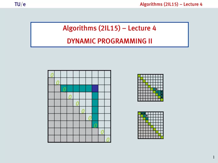
Algorithms (2IL15) Lecture 4 DYNAMIC PROGRAMMING II 0 0 0 0 0 - PowerPoint PPT Presentation

TU/e Algorithms (2IL15) – Lecture 4 Algorithms (2IL15) – Lecture 4 DYNAMIC PROGRAMMING II 0 0 0 0 0 0 0 0 0 0 1

TU/e Algorithms (2IL15) – Lecture 4 Techniques for optimization optimization problems typically involve making choices backtracking: just try all solutions  can be applied to almost all problems, but gives very slow algorithms  try all options for first choice, for each option, recursively make other choices greedy algorithms: construct solution iteratively, always make choice that seems best  can be applied to few problems, but gives fast algorithms  only try option that seems best for first choice (greedy choice), recursively make other choices dynamic programming  in between: not as fast as greedy, but works for more problems 2

TU/e Algorithms (2IL15) – Lecture 4 5 steps in designing dynamic-programming algorithms 1. define subproblems [#subproblems] 2. guess first choice [#choices] 3. give recurrence for the value of an optimal solution [time/subproblem treating recursive calls as Θ (1))] i. define subproblem in terms of a few parameters Today more examples: ii. define variable m [..] = value of optimal solution for subproblem longest common subsequence and optimal binary search trees iii. relate subproblems by giving recurrence for m [..] 4. algorithm: fill in table for m [..] in suitable order (or recurse & memoize) 5. solve original problem Running time: #subproblems * time/subproblem Correctness: (i) correctness of recurrence: relate OPT to recurrence (ii) correctness of algorithm: induction using (i) 3

TU/e Algorithms (2IL15) – Lecture 4 5 steps: Matrix chain multiplication [ Θ (n 2 )] 1. define subproblems given i,j with 1 ≤ i<j ≤ n , compute A i • … • A j in cheapest way 2. guess first choice final multiplication [ Θ (n)] 3. give recurrence for the value of an optimal solution m [ i,j ] = 0 if i = j [ Θ (n)] min { m [ i,k ] + m [ k+1,j ] + p i-1 p k p j } if i< j i ≤k<j 4. algorithm: fill in table for m [..] in suitable order (or recurse & memoize) Blackboard example 5. solve original problem: split markers s[i,j] Running time: #subproblems * time/subproblem = Θ (n 3 ) 4

TU/e Algorithms (2IL15) – Lecture 4 Longest Common Subsequence 5

TU/e Algorithms (2IL15) – Lecture 4 Comparing DNA sequences DNA: string of characters A = adenine C = cytosine G = guanine T = thymine Problem: measure the similarity of two given DNA sequences X = A C C G T A A T C G A C G Y = A C G A T T G C A C T G How to measure similarity?  edit distance: number of changes to transform X into Y  length of longest common subsequence (LCS) of X and Y  … 6

TU/e Algorithms (2IL15) – Lecture 4 Longest common subsequence substring of a string: string that can be obtained by omitting zero or more characters string: A C C A T T G example substrings: A C C A T T G or A C C A T T G or … LCS(X,Y) = a longest common subsequence of strings X and Y = a longest string that is a subsequence of X and a subsequence of Y X = A C C G T A A T C G A C G Y = A C G A T T G C A C T G LCS( X,Y ) = ACGTTGACG (or ACGTTCACG …) 7

TU/e Algorithms (2IL15) – Lecture 4 The LCS problem Input: strings X = x 1 , x 2 , … , x n and Y = y 1 , y 2 , … , y m Output: (the length of) a longest common subsequence of X and Y So we have valid solution = common subsequence profit = length of the subsequence (to be maximized) 8

TU/e Algorithms (2IL15) – Lecture 4 Let’s study the structure of an optimal solution  what are the choices that need to be made?  what are the subproblems that remain? do we have optimal substructure? x 1 x 2 x n optimal solution X = A C C G T A A T C G A C G Y = A C G A T T G C A C T G y 1 y 2 y m first choice: is last character of X matched to last character of Y ? LCS for x 1 …x n-1 and y 1 …y m-1 or is last character of X unmatched ? so: optimal substructure or is last character of Y unmatched ? greedy choice ? overlapping subproblems ? 9

TU/e Algorithms (2IL15) – Lecture 4 5 steps in designing dynamic-programming algorithms 1. define subproblems 2. guess first choice 3. give recurrence for the value of an optimal solution 4. algorithm: fill in table for c [..] in suitable order (or recurse & memoize) 5. solve original problem 10

TU/e Algorithms (2IL15) – Lecture 4 3. Give recursive formula for the value of an optimal solution i. define subproblem in terms of a few parameters Find LCS of X i := x 1 … x i and Y j := y 1 … y j , for parameters i, j with 0 ≤ i ≤ n and 0 ≤ j ≤ m ? X 0 is empty string ii. define variable c [..] = value of optimal solution for subproblem c [ i,j ] = length of LCS of X i and Y j iii. give recursive formula for c [..] x 1 x 2 x n X = A C C G T A A T C G A C G Y = A C G A T T G C A C T G y 1 y 2 y m 11

TU/e Algorithms (2IL15) – Lecture 4 X i := x 1 … x i and Y j := y 1 … y j , for 0 ≤ i ≤ n and 0 ≤ j ≤ m we want recursive formula for c [ i,j ] = length of LCS of X i and Y j x 1 x 2 x n X = A C C G T A A T C G A C G Y = A C G A T T G C A C T G y 1 y 2 y m 0 Lemma: c [ i,j ] = if i = 0 or j = 0 c[i-1,j-1] + 1 if i,j > 0 and x i = y j if i,j > 0 and x i ≠ y j max { c[i-1,j], c[i,j-1] } 12

TU/e Algorithms (2IL15) – Lecture 4 0 Lemma: c [ i,j ] = if i = 0 or j = 0 c[i-1,j-1] + 1 if i,j > 0 and x i = y j if i,j > 0 and x i ≠ y j max { c[i-1,j], c[i,j-1] } Proof: i =0 or j = 0: trivial (at least one of X i and Y j is empty) i,j > 0 and x i = y j : We can extend LCS ( X i-1 , Y j-1 ) by appending x i , so c [ i,j ] ≥ c [ i-1,j-1 ] + 1. On the other hand, by deleting the last character from LCS( X i , Y j ) we obtain a substring of X i-1 and Y j-1 . Hence, c [ i-1,j-1 ] ≥ c [ i,j ] - 1. It follows that c [ i,j ] = c [ i-1,j-1 ] + 1. i,j > 0 and x i ≠ y j : If LCS( X i , Y j ) does not end with x i then c [ i,j ] ≤ c [ i-1,j ] ≤ max { .. }. Otherwise LCS( X i , Y j ) cannot end with y j , so c [ i,j ] ≤ c [ i,j-1 ] ≤ max { .. }. Obviously c [ i,j ] ≥ max { .. } . We conclude that c [ i,j ] = max { .. }. 13

TU/e Algorithms (2IL15) – Lecture 4 5 steps in designing dynamic-programming algorithms 1. define subproblems 2. guess first choice 3. give recurrence for the value of an optimal solution 4. algorithm: fill in table for c [..] in suitable order (or recurse & memoize) 5. solve original problem 14

TU/e Algorithms (2IL15) – Lecture 4 4. Algorithm: fill in table for c [..] in suitable order 0 c [ i,j ] = if i = 0 or j = 0 c[i-1,j-1] + 1 if i,j > 0 and x i = y j if i,j > 0 and x i ≠ y j max { c[i-1,j], c[i,j-1] } j 0 m 0 0 0 0 0 0 0 0 0 0 0 0 0 0 solution to original problem 0 i 0 0 0 0 n 0 15

TU/e Algorithms (2IL15) – Lecture 4 4. Algorithm: fill in table for c [..] in suitable order 0 c [ i,j ] = if i = 0 or j = 0 c[i-1,j-1] + 1 if i,j > 0 and x i = y j if i,j > 0 and x i ≠ y j max { c[i-1,j], c[i,j-1] } LCS-Length ( X,Y ) j 0 m 1. n ← length[X]; m ← length[Y] 0 2. for i ← 0 to n do c[i,0] ← 0 3. for j ← 0 to m do c[0,j] ← 0 i 4. for i ← 1 to n 5. do for j ← 1 to m n 6. do if X[i] = Y[j] 7. then c[i,j] ← c[i -1,j-1] + 1 8. else c[i,j] ← max { c[i-1,j], c[i,j-1] } 9. return c[n,m] 16

TU/e Algorithms (2IL15) – Lecture 4 Analysis of running time LCS-Length ( X,Y ) Θ (1) 1. n ← length[X]; m ← length[Y] Θ (n) 2. for i ← 0 to n do c[i,0] ← 0 Θ (m) 3. for j ← 0 to m do c[0,j] ← 0 4. for i ← 1 to n 5. do for j ← 1 to m 6. do if X[i] = Y[j] 7. then c[i,j] ← c[i -1,j-1] + 1 8. else c[i,j] ← max { c[i-1,j], c[i,j-1] } Θ (1) 9. return c[n,m] Lines 4 – 8: ∑ 1≤i≤n ∑ 1≤j≤m Θ (1) = Θ (nm) 17

TU/e Algorithms (2IL15) – Lecture 4 5 steps in designing dynamic-programming algorithms 1. define subproblems 2. guess first choice 3. give recurrence for the value of an optimal solution 4. algorithm: fill in table for c [..] in suitable order (or recurse & memoize) 5. solve original problem Approaches for going from optimum value to optimum solution: i. store choices that led to optimum (e.g. s[i,j] for matrix multiplication) ii. retrace/deduce sequence of solutions that led to optimum backwards (next slide) 18

TU/e Algorithms (2IL15) – Lecture 4 5. Extend algorithm so that it computes an actual solution that is optimal, and not just the value of an optimal solution. Usual approach: extra table to remember choices that lead to optimal solution It’s also possible to do without the extra table. Print-LCS(c,X,Y,i,j) Initial call: Print-LCS(c,X,Y,n,m) 1. if i=0 or j=0 2. then skip 3. else if X[i] = Y[j] 4. then Print-LCS(c,X,Y,i-1,j-1); print x i 5. else if c[i-1,j] > c[i,j-1] 6. then Print-LCS(c,X,Y,i-1,j) 7. else Print-LCS (c,X,Y,i,j-1) Advantage of avoiding extra table: saves memory Disadvantage: extra work to construct solution 19