Dynamic Programming Outline and Reading Matrix Chain-Product - PowerPoint PPT Presentation

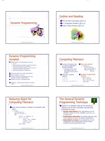
Dynamic Programming

Outline and Reading • Matrix Chain-Product (5.3.1) • Dynamic Programming: The General Technique (5.3.2) • 0-1 Knapsack Problem (5.3.3) Dynamic Programming 2

Matrix Chain Product Dynamic Programming is a general algorithm design paradigm. • Rather than give the general structure, we first give a motivating example: Matrix Chain-Product f B Review: Matrix Multiplication • C = A * B j e • A is d × e and B is e × f - e 1 å = C [ i , j ] A [ i , k ] * B [ k , j ] e = k 0 A C d i i,j d O ( d × e × f ) time • f Dynamic Programming 3

Matrix Chain Product Matrix Chain-Product : • Compute A=A 0 *A 1 *…*A n-1 A i is d i × d i+1 • • Problem : How to parenthesize in such a way that minimizes the total number of scalar multiplications? Example: B is 3 × 100 • C is 100 × 5 • D is 5 × 5 • • (B*C)*D takes 1500 + 75 = 1575 ops • B*(C*D) takes 1500 + 2500 = 4000 ops Dynamic Programming 4

Another Approach: Greedy (v1) Idea: Repeatedly select the product that uses (up) the most operations. Counter-example: A is 10 × 5 • B is 5 × 10 • C is 10 × 5 • D is 5 × 10 • This greedy approach gives (A*B)*(C*D) • takes 500+1000+500 = 2000 ops A better solution: A*((B*C)*D) • takes 500+250+250 = 1000 ops Dynamic Programming 5

Another Approach: Greedy (v2) Idea: Repeatedly select the product that uses the fewest operations. Counter-example: A is 101 × 11 • B is 11 × 9 • C is 9 × 100 • D is 100 × 99 • This greedy approach gives A*((B*C)*D)) • takes 109989+9900+108900=228789 ops A better solution is (A*B)*(C*D) • takes 9999+89991+89100=189090 ops The greedy approach is not giving us the optimal value. 6

“Recursive” Approach Define subproblems: • Find the best parenthesization of A i *A i+1 *…*A j . • Let N i,j denote the number of operations done by this subproblem. • The optimal solution for the whole problem is N 0,n-1 . Subproblem optimality : The optimal solution can be defined in terms of optimal subproblems • There has to be a final multiplication (root of the expression tree) for the optimal solution. • Say, the final multiply is at index i: (A 0 *…*A i )*(A i+1 *…*A n-1 ). • Then the optimal solution N 0,n-1 is the sum of two optimal subproblems, N 0,i and N i+1,n-1 plus the time for the last multiply. • If the global optimum did not have these optimal subproblems, we could define an even better “ optimal ” solution. Dynamic Programming 7

Characterizing Equation • The global optimal has to be defined in terms of optimal subproblems, depending on where the final multiply is at. • Consider all possible places for that final multiply: – Recall that A i is a d i × d i+1 dimensional matrix. – So, a characterizing equation for N i,j is the following: = + + N min { N N d d d } + + + i , j i , k k 1 , j i k 1 j 1 £ < i k j • Note that subproblems are not independent – meaning subproblems overlap. Dynamic Programming 8

Dynamic Programming Algorithm Visualization = + + N min { N N d d d } The bottom-up construction fills in + + + i , j i , k k 1 , j i k 1 j 1 £ < i k j the N array by diagonals N 0 1 2 i j … n-1 N i,j gets values from previous 0 entries in i-th row and j-th column 1 answer … i Filling in each entry in the N table takes O(n) time. • Total run time: O(n 3 ) j Getting actual parenthesization can n-1 be done by remembering “ k ” for each N entry in a separate table Dynamic Programming 9

Dynamic Programming Algorithm Since subproblems Algorithm matrixChain ( S ): overlap, we don’t use Input: sequence S of n matrices to be multiplied recursion. Output: number of operations in an optimal parenthesization of S Instead, we construct for i ¬ 0 to n - 1 do optimal subproblems N i,i ¬ 0 “ bottom-up. ” for length ¬ 1 to n - 1 do { length = j - i is the length of the chain } N i,i ’ s are easy, so start for i ¬ 0 to n – 1 - length do with them j ¬ i + length N i,j ¬ + ¥ Then do problems of “ length ” 2,3,… for k ¬ i to j - 1 do subproblems, and so on. N i,j ¬ min{ N i,j , N i,k + N k+ 1 ,j + d i d k+ 1 d j+ 1 } record k that produces minimum N i,j Running time: O(n 3 ) return N 0, n - 1 10

matrix: dimension: 30x35 35x15 15x5 5x10 10x20 20x25 Dynamic Programming 11

matrix: dimension: 30x35 35x15 15x5 5x10 10x20 20x25 end j k 0 1 2 3 4 5 N 0 1 2 3 4 5 0 0 0 1 1 0 start 2 2 0 i 3 0 3 4 4 0 5 5 0 number of scalar operations required to multiply matrix index where final multiplication occurred to obtain optimal solution given in N[i][j] 12

matrix: dimension: 30x35 35x15 15x5 5x10 10x20 20x25 end j k 0 1 2 3 4 5 N 0 1 2 3 4 5 0 0 0 0 15750 1 1 0 start 2 2 0 i 3 0 3 4 4 0 5 5 0 number of scalar operations required to multiply matrix index where final multiplication occurred to obtain optimal solution given in N[i][j] N[0][1] = 0 + 0 + 30*35*15 = 15750 13

matrix: dimension: 30x35 35x15 15x5 5x10 10x20 20x25 end j k 0 1 2 3 4 5 N 0 1 2 3 4 5 0 0 0 0 15750 1 1 1 0 2625 start 2 2 0 i 3 0 3 4 4 0 5 5 0 number of scalar operations required to multiply matrix index where final multiplication occurred to obtain optimal solution given in N[i][j] N[0][1] = 0 + 0 + 30*35*15 = 15750 N[1][2] = 0 + 0 + 35*15*5 = 2626 14

matrix: dimension: 30x35 35x15 15x5 5x10 10x20 20x25 end j k 0 1 2 3 4 5 N 0 1 2 3 4 5 0 0 0 0 15750 1 1 1 0 2625 start 2 2 2 0 750 i 3 0 3 4 4 0 5 5 0 number of scalar operations required to multiply matrix index where final multiplication occurred to obtain optimal solution given in N[i][j] N[0][1] = 0 + 0 + 30*35*15 = 15750 N[1][2] = 0 + 0 + 35*15*5 = 2626 N[2][3] = 0 + 0 + 15*5*10 = 750 15

matrix: dimension: 30x35 35x15 15x5 5x10 10x20 20x25 end j k 0 1 2 3 4 5 N 0 1 2 3 4 5 0 0 0 0 15750 1 1 1 0 2625 start 2 2 2 0 750 i 3 0 1000 3 3 4 4 0 5 5 0 number of scalar operations required to multiply matrix index where final multiplication occurred to obtain optimal solution given in N[i][j] N[0][1] = 0 + 0 + 30*35*15 = 15750 N[1][2] = 0 + 0 + 35*15*5 = 2626 N[2][3] = 0 + 0 + 15*5*10 = 750 N[3][4] = 0 + 0 + 5*10*20 = 1000 16

matrix: dimension: 30x35 35x15 15x5 5x10 10x20 20x25 end j k 0 1 2 3 4 5 N 0 1 2 3 4 5 0 0 0 0 15750 1 1 1 0 2625 start 2 2 2 0 750 i 3 0 1000 3 3 4 4 4 0 5000 5 5 0 number of scalar operations required to multiply matrix index where final multiplication occurred to obtain optimal solution given in N[i][j] N[0][1] = 0 + 0 + 30*35*15 = 15750 N[1][2] = 0 + 0 + 35*15*5 = 2626 N[2][3] = 0 + 0 + 15*5*10 = 750 N[3][4] = 0 + 0 + 5*10*20 = 1000 N[4][5] = 0 + 0 + 10*20*25 = 5000 17

matrix: dimension: 30x35 35x15 15x5 5x10 10x20 20x25 end j k 0 1 2 3 4 5 N 0 1 2 3 4 5 0 0 0 0 0 15750 7875 1 1 1 0 2625 start 2 2 2 0 750 i 3 0 1000 3 3 4 4 4 0 5000 5 5 0 = 0 + 2625 + 30*35*5 = 7875 = 15750 + 0 + 30*15*5 = 18000 18

matrix: dimension: 30x35 35x15 15x5 5x10 10x20 20x25 end j k 0 1 2 3 4 5 N 0 1 2 3 4 5 0 0 0 0 0 15750 7875 1 1 2 1 0 2625 4375 start 2 2 2 0 750 i 3 0 1000 3 3 4 4 4 0 5000 5 5 0 = 0 + 750 + 35*15*10 = 6000 = 2625 + 0 + 35*5*10 = 4375 19

matrix: dimension: 30x35 35x15 15x5 5x10 10x20 20x25 end j k 0 1 2 3 4 5 N 0 1 2 3 4 5 0 0 0 0 0 15750 7875 1 1 2 1 0 2625 4375 start 2 2 2 2 0 750 2500 i 3 0 1000 3 3 4 4 4 0 5000 5 5 0 = 0 + 1000 + 15*5*20 = 2500 = 750 + 0 + 15*10*20 = 3750 20

matrix: dimension: 30x35 35x15 15x5 5x10 10x20 20x25 end j k 0 1 2 3 4 5 N 0 1 2 3 4 5 0 0 0 0 0 15750 7875 1 1 2 1 0 2625 4375 start 2 2 2 2 0 750 2500 i 3 0 1000 3500 3 3 4 4 4 4 0 5000 5 5 0 = 0 + 5000 + 5*10*25 = 6250 = 1000 + 0 + 5*20*25 = 3500 21

matrix: dimension: 30x35 35x15 15x5 5x10 10x20 20x25 end j k 0 1 2 3 4 5 N 0 1 2 3 4 5 0 0 0 2 0 0 15750 7875 9375 1 1 2 1 0 2625 4375 start 2 2 2 2 0 750 2500 i 3 0 1000 3500 3 3 4 4 4 4 0 5000 5 5 0 = 0 + 4375 + 30*35*10 = 14875 = 15750 + 750 + 30*15*10 = 21000 = 7875 + 0 + 30*5*10 = 9375 22

matrix: dimension: 30x35 35x15 15x5 5x10 10x20 20x25 end j k 0 1 2 3 4 5 N 0 1 2 3 4 5 0 0 0 2 0 0 15750 7875 9375 1 1 2 2 1 0 2625 4375 7125 start 2 2 2 2 0 750 2500 i 3 0 1000 3500 3 3 4 4 4 4 0 5000 5 5 0 = 0 + 2500 + 35*15*20 = 13000 = 2625 + 1000 + 35*5*20 = 7125 = 4375 + 0 + 35*10*20 = 11375 23