Dynamic Programming (Chapter 6) Algorithm Design Techniques - PowerPoint PPT Presentation

Dynamic Programming (Chapter 6)

Algorithm Design Techniques Greedy Divide and Conquer Dynamic Programming Network Flows

Algorithm Design Divide and Dynamic Greedy Conquer Programming Formulate problem ? ? ? Design algorithm less work more work more work Prove correctness more work less work less work Analyze running time less work more work less work

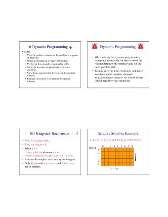
Dynamic Programming “Recipe” Recursive formulation of optimal solution in terms of subproblems Obvious implementation requires solving exponentially many subproblems Careful implementation to solve only polynomially many different subproblems

Interval Scheduling (Yes, this is an old problem!) Job j starts at s j and finishes at f j . Two jobs compatible if they don't overlap. Goal: find maximum subset of mutually compatible jobs. a b c d e f g h Time 0 1 2 3 4 5 6 7 8 9 10 11

Interval Scheduling: Greedy Solution Sort jobs by earliest finish time. Take each job provided it's compatible with the ones already taken. a b b, e, h c d e f g h Time 0 1 2 3 4 5 6 7 8 9 10 11

Weighted Interval Scheduling Job j starts at s j , finishes at f j , and has weight v j . Two jobs compatible if they don't overlap. Goal: find maximum weight subset of mutually compatible jobs. 3 2 4 1 3 4 3 1 Time 0 1 2 3 4 5 6 7 8 9 10 11

Greedy Solution? Observation. Greedy algorithm can be arbitrarily bad when intervals are weighted. weight = 999 weight = 1 Time 0 1 2 3 4 5 6 7 8 9 10 11

Weighted Interval Scheduling Label jobs by finishing time: f 1 ≤ f 2 ≤ . . . ≤ f n . p(j) = largest index i < j such that job i is compatible with j. E.g.: p(8) = 5, p(7) = 5, p(2) = 0. 1 3 2 2 3 4 4 1 5 3 6 4 7 3 8 1 Time 0 1 2 3 4 5 6 7 8 9 10 11

Dynamic Programming: Binary Choice OPT(j) = value of optimal solution to the problem consisting of job requests 1, 2, ..., j. Case 1: OPT selects job j. Case 2: OPT does not select job j.

If OPT selects job j... can't use incompatible jobs { p(j) + 1, p(j) + 2, ..., j - 1 } must include optimal solution to problem consisting of remaining compatible jobs 1, 2, ..., p(j) 1 3 2 2 3 4 4 1 5 3 6 5 p(j) + 1, p(j) + 2, ..., j - 1 7 2 8 1 Time 0 1 2 3 4 5 6 7 8 9 10 11

If OPT does not select job j... must include optimal solution to problem consisting of remaining compatible jobs 1, 2, ..., j-1 1 3 2 2 3 4 4 1 5 3 6 4 7 3 8 1 Time 0 1 2 3 4 5 6 7 8 9 10 11

Optimal Substructure OPT(j) = value of optimal solution to the problem consisting of job requests 1, 2, ..., j Case 1: OPT selects job j Case 2: OPT does not select job j Recurrence for OPT(j) ⎧ if j = 0 0 OPT ( j ) = ⎨ { } v j + OPT ( p ( j )), OPT ( j − 1) ⎩ max otherwise Case 1 Case 2

Straightforward Recursive Algorithm Sort jobs by finish time: f 1 ≤ f 2 ≤ ... ≤ f n . Compute p(1), p(2), …, p(n) Compute-Opt(j) { if (j = 0) return 0 else return max(v j + Compute-Opt(p(j)), Compute-Opt(j-1)) } Running time?

Worst Case Running Time 5 4 3 1 2 3 2 2 1 3 4 2 1 1 0 1 0 5 1 0 p(1) = 0, p(j) = j-2 Worst-case is exponential How can we do better?

Memoization Memoization. Store results of each sub-problem in an array; lookup as needed. Sort jobs by finish times so that f 1 ≤ f 2 ≤ ... ≤ f n . Compute p(1), p(2), …, p(n) for j = 1 to n M[j] = empty M[0] = 0 M-Compute-Opt(j) { if (M[j] is empty) M[j] = max(w j + M-Compute-Opt(p(j)), M-Compute-Opt(j-1)) return M[j] }

Memoization 1 3 2 2 3 4 4 1 3 5 6 4 7 3 8 1 Time 0 1 2 3 4 5 6 7 8 9 10 11 M M[8] = max(1 + M-Compute-Opt(5), M-Compute-Opt(7)

Memoization 1 3 2 2 3 4 4 1 3 5 6 4 7 3 8 1 Time 0 1 2 3 4 5 6 7 8 9 10 11 M M[5] = max(3 + M-Compute-Opt(2), M-Compute-Opt(4)

Memoization 1 3 2 2 3 4 4 1 3 5 6 4 7 3 8 1 Time 0 1 2 3 4 5 6 7 8 9 10 11 M M[2] = max(2 + 0, M-Compute-Opt(1)

Memoization 1 3 2 2 3 4 4 1 3 5 6 4 7 3 8 1 Time 0 1 2 3 4 5 6 7 8 9 10 11 3 M M[1] = max(3 + 0, 0)

Memoization 1 3 2 2 3 4 4 1 3 5 6 4 7 3 8 1 Time 0 1 2 3 4 5 6 7 8 9 10 11 3 3 M M[2] = max(2 + 0, 3)

Memoization 1 3 2 2 3 4 4 1 3 5 6 4 7 3 8 1 Time 0 1 2 3 4 5 6 7 8 9 10 11 3 3 M M[5] = max(3 + 3, M-Compute-Opt(4)

Memoization 1 3 2 2 3 4 4 1 3 5 6 4 7 3 8 1 Time 0 1 2 3 4 5 6 7 8 9 10 11 3 3 M M[4] = max(1 + 3, M-Compute-Opt(3)

Memoization 1 3 2 2 3 4 4 1 3 5 6 4 7 3 8 1 Time 0 1 2 3 4 5 6 7 8 9 10 11 3 3 4 M M[3] = max(4 + 0, 3)

Memoization 1 3 2 2 3 4 4 1 3 5 6 4 7 3 8 1 Time 0 1 2 3 4 5 6 7 8 9 10 11 3 3 4 4 M M[4] = max(1 + 3, 4)

Memoization 1 3 2 2 3 4 4 1 3 5 6 4 7 3 8 1 Time 0 1 2 3 4 5 6 7 8 9 10 11 3 3 4 4 6 M M[5] = max(3 + 3, 4)

Memoization 1 3 2 2 3 4 4 1 3 5 6 4 7 3 8 1 Time 0 1 2 3 4 5 6 7 8 9 10 11 3 3 4 4 6 M M[8] = max(1 + 6, M-Compute-Opt(7)

Memoization 1 3 2 2 3 4 4 1 3 5 6 4 7 3 8 1 Time 0 1 2 3 4 5 6 7 8 9 10 11 3 3 4 4 6 M M[7] = max(3 + 6, M-Compute-Opt(6))

Memoization 1 3 2 2 3 4 4 1 3 5 6 4 7 3 8 1 Time 0 1 2 3 4 5 6 7 8 9 10 11 3 3 4 4 6 8 M M[6] = max(4 + 4, 6)

Memoization 1 3 2 2 3 4 4 1 3 5 6 4 7 3 8 1 Time 0 1 2 3 4 5 6 7 8 9 10 11 3 3 4 4 6 8 9 M M[7] = max(3 + 6, 8)

Memoization 1 3 2 2 3 4 4 1 3 5 6 4 7 3 8 1 Time 0 1 2 3 4 5 6 7 8 9 10 11 3 3 4 4 6 8 9 9 M M[8] = max(1 + 6, 9)

Memoization 1 3 2 2 3 4 4 1 3 5 6 4 7 3 8 1 Time 0 1 2 3 4 5 6 7 8 9 10 11 3 3 4 4 6 8 9 9 M

Running Time? Sort jobs by finish times so that f 1 ≤ f 2 ≤ ... ≤ f n . Compute p(1), p(2), …, p(n) for j = 1 to n M[j] = empty M[0] = 0 M-Compute-Opt(j) { if (M[j] is empty) M[j] = max(w j + M-Compute-Opt(p(j)), M-Compute-Opt(j-1)) return M[j] }

Iterative Solution Bottom-up dynamic programming. Solve subproblems in ascending order. Sort jobs by finish time: f 1 ≤ f 2 ≤ ... ≤ f n . Compute p(1), p(2), …, p(n) Iterative-Compute-Opt { M[0] = 0 for j = 1 to n M[j] = max(v j + M[p(j)], M[j-1]) }

Compute the Solution (Not Just Its Value) Exercise: suppose you know the value OPT(j) for all j. How can you produce the set of intervals in the optimal solution?

Dynamic Programming “Recipe” Recursive formulation of optimal solution in terms of subproblems Obvious implementation requires solving exponentially many subproblems Careful implementation to solve only polynomially many different subproblems