Algorithms and Data Structures Lecture 11 Dynamic Programming - PowerPoint PPT Presentation
Algorithms and Data Structures Lecture 11 Dynamic Programming Fabian Kuhn Algorithms and Complexity Fabian Kuhn Algorithms and Data Structures Dynamic Programming (DP) Important algorithm design technique! Simple, but very often a
Algorithms and Data Structures Lecture 11 Dynamic Programming Fabian Kuhn Algorithms and Complexity Fabian Kuhn Algorithms and Data Structures
Dynamic Programming (DP) • Important algorithm design technique! • Simple, but very often a very effective idea • Many problems that naively require exponential time can be solved in polynomial time by using dynamic programming. – This in particular holds for optimization problems (min / max) DP ≈ careful / optimized brute force solution DP ≈ recursion + reuse of partial solutions Fabian Kuhn Algorithms and Data Structures 2
DP: History • Where does the name come from? • DP was developed by Richard E. Bellman in the 1940s and 1950s. In his autobiography, he writes: "I spent the Fall quarter (of 1950) at RAND. My first task was to find a name for multistage decision processes. … The 1950s were not good years for mathematical research. We had a very interesting gentleman in Washington named Wilson. He was Secretary of Defense, and he actually had a pathological fear and hatred of the word research. … His face would suffuse, he would turn red, and he would get violent if people used the term research in his presence. You can imagine how he felt, then, about the term mathematical. … Hence , I felt I had to do something to shield Wilson and the Air Force from the fact that I was really doing mathematics inside the RAND Corporation. What title, what name, could I choose? In the first place I was interested in planning, in decision making, in thinking. But planning, is not a good word for various reasons. I decided therefore to use the word “programming”. I wanted to get across the idea that this was dynamic, this was multistage, this was time-varying. … It also has a very interesting property as an adjective, and that it's impossible to use the word dynamic in a pejorative sense. … Thus, I thought dynamic programming was a good name. It was something not even a Congressman could object to. …“ Fabian Kuhn Algorithms and Data Structures 3
Fibonacci Numbers Definition of the Fibonacci numbers 𝑮 𝟏 , 𝑮 𝟐 , 𝑮 𝟑 , … : 𝐺 0 = 0, 𝐺 1 = 1 𝐺 𝑜 = 𝐺 𝑜−1 + 𝐺 𝑜−2 Goal: Compute 𝐺 𝑜 • This can easily be done recursively… def fib(n): if n < 2: f = n else: f = fib(n-1) + fib(n-2) return f Fabian Kuhn Algorithms and Data Structures 4
Running Time of Recursive Algorithm def fib(n): if n < 2: f = n else: f = fib(n-1) + fib(n-2) return f fib(n) fib(n-2) fib(n-1) fib(n-4) fib(n-3) fib(n-3) fib(n-2) fib(n-6) fib(n-5) fib(n-5) fib(n-4) fib(n-5) fib(n-4) fib(n-4) fib(n-3) • Recursion tree is a binary tree that is complete up to depth Τ 𝑜 2 . • Running time : Ω 2 Τ 𝑜 2 – We repeatedly compute the same things! Fabian Kuhn Algorithms and Data Structures 5
Algorithm with Memoization Memoization: One stores already computed values (on a notepad = memo) creates a new dictionary memo = {} (a hash table) def fib(n): First check,if we have if n in memo: return memo[n] already computed fib(n) . if n < 2: f = n else: f = fib(n-1) + fib(n-2) Store the computed value for memo[n] = f fib(n) in the hash table. return f • Now, each value fib(i) is only computed once recursively – For every 𝑗 we only go once through the blue part. – The recursion tree therefore has ≤ 𝑜 inner nodes. – The running time is therefore 𝑃 𝑜 . Fabian Kuhn Algorithms and Data Structures 6
DP: A bit more precisely … DP ≈ Recursion + Memoization Memoize: Store solutions for subproblems , reuse stored solutions if the same subproblem appears again. • For the Fibonacci numbers, the subproblems are 𝐺 0 , 𝐺 1 , 𝐺 2 , … Running Time = #subproblems ⋅ time per subproblem Usually just the number of recursive calls per subproblem. Fabian Kuhn Algorithms and Data Structures 7
Fibonacci: Bottom-Up def fib(n): fn = {} for k in [0,1, 2, …, n]: if k < 2: f = k else: f = fn[k-1] + fn[k-2] fn[k] = f return fn[n] • Go through the subproblms in an order such that one has always already computed the subproblems that one needs. – In the case of the Fibonacci numbers, compute 𝐺 𝑗−2 and 𝐺 𝑗−1 , before computing 𝐺 𝑗 . Fabian Kuhn Algorithms and Data Structures 8
Shortest Paths with DP • Given: weighted, directed graph 𝐻 = 𝑊, 𝐹, 𝑥 – starting node 𝑡 ∈ 𝑊 – We denote the weight of an edge 𝑣, 𝑤 as 𝑥 𝑣, 𝑤 – Assumption: ∀𝑓 ∈ 𝐹: 𝑥 𝑓 , no negative cycles • Goal: Find shortest paths / distances from 𝑡 to all nodes – Distance from 𝑡 to 𝑤 : 𝑒 𝐻 𝑡, 𝑤 (length of a shortest path) 1 𝑡 1 15 3 3 9 7 11 3 4 2 6 6 1 9 8 17 10 9 Fabian Kuhn Algorithms and Data Structures 9
Shortest Paths : Recursive Formulation Recursive characterization of 𝒆 𝑯 𝒕, 𝒘 ? • How does a shortest path from 𝑡 to 𝑤 look like? • Optimality of subpaths: If 𝑤 ≠ 𝑡 , then there is a node 𝑣 , such that the shortest path consists of a shortest path from 𝑡 to 𝑣 and the edge 𝑣, 𝑤 . 𝒕 𝒗 𝒘 shortest path ∀𝒘 ≠ 𝒕 ∶ 𝒆 𝑯 𝒕, 𝒘 = 𝒗∈𝑶 𝐣𝐨 (𝒘) 𝒆 𝑯 𝒕, 𝒗 + 𝒙 𝒗, 𝒘 𝐧𝐣𝐨 • Can we use this to compute the values 𝑒 𝐻 𝑡, 𝑤 recursively? Fabian Kuhn Algorithms and Data Structures 10
Shortest Paths : Recursive Formulation Recursive characterization of 𝒆 𝑯 (𝒕, 𝒘) ? 𝑒 𝐻 𝑡, 𝑤 = 𝑣∈𝑂 in (𝑤) 𝑒 𝐻 𝑡, 𝑣 + 𝑥 𝑣, 𝑤 min , 𝑒 𝐻 𝑡, 𝑡 = 0 dist(v): d = ∞ if v == s: d = 0 else: for (u,v) in E: d = min(d, dist(u) + w(u,v)) return d Problem: cycles! • With cycles we obtain an infinite recursion – Example: Cycle of length 2 (edges 𝑣, 𝑤 and 𝑤, 𝑣 ) – dist(v) calls dist(u) , dist(u) then again calls dist(v) , etc. Fabian Kuhn Algorithms and Data Structures 11
Shortest Paths in Acyclic Graphs memo = {} dist(v): if v in memo: return memo[v] d = ∞ if v == s: d = 0 else: (go through all incoming edges of v) for (u,v) in E: d = min(d, dist(u) + w(u,v)) memo[v] = d return d Running time: 𝑷 𝒏 • Number of subproblems: 𝑜 • Time for subproblem 𝑒 𝐻 𝑡, 𝑤 : #incoming edges of 𝑤 Fabian Kuhn Algorithms and Data Structures 12
Acyclic Graphs: Bottom-Up Observation: • Edge 𝑣, 𝑤 ⟹ 𝑒 𝐻 𝑡, 𝑣 must be computed before 𝑒 𝐻 𝑡, 𝑤 • One can first compute a topological sort of the nodes. Assumption: • Sequence 𝑤 1 , 𝑤 2 , … , 𝑤 𝑜 is a topological sort of the nodes. D = “array of length n” for i in [1:n]: D[i] = ∞ if 𝑤 𝑗 == 𝑡 : D[i] = 0 else: for (𝑤 𝑘 , 𝑤 𝑗 ) in 𝐹 : (incoming edges, top. sort ⟹ 𝑘 < 𝑗 ) D[i] = min(D[i], D[j] + 𝑥(𝑤 𝑘 , 𝑤 𝑗 ) ) Fabian Kuhn Algorithms and Data Structures 13
Shortest Paths in General Graphs Idea: Introduce additional subproblems to avoid cyclic dependencies 𝒍 𝒕, 𝒘 Subproblems 𝒆 𝑯 • Length of shortest path consisting of at most 𝑙 edges Recursive Definition: 𝑙 𝑡, 𝑤 = min 𝑒 𝐻 𝑙−1 𝑡, 𝑤 , min 𝑙−1 𝑡, 𝑣 + 𝑥(𝑣, 𝑤) 𝑒 𝐻 𝑣,𝑤 ∈𝐹 𝑒 𝐻 𝑙 𝑡, 𝑡 = 0, 𝑒 𝐻 (∀𝑙 ≥ 0) 0 𝑡, 𝑤 = ∞, 𝑒 𝐻 (∀𝑤 ≠ 𝑡) Fabian Kuhn Algorithms and Data Structures 14
Shortest Paths in General Graphs memo = {} dist(k, v): if (k, v) in memo: return memo[(k, v)] d = ∞ if s == v: d = 0 elif k > 0: d = dist(k-1, v) for (u,v) in E: (go through all incoming edges of v) d = min(d, dist(k-1, u) + w(u,v)) memo[(k, v)] = d return d distance(v): return dist(n-1, v) Fabian Kuhn Algorithms and Data Structures 15
Shortest Paths with DP: Running Time DP running time, typically: #𝐭𝐯𝐜𝐪𝐬𝐩𝐜𝐦𝐟𝐧𝐭 ⋅ 𝐮𝐣𝐧𝐟 𝐪𝐟𝐬 𝐭𝐯𝐜𝐪𝐬𝐩𝐜𝐦𝐟𝐧 • Time per subproblem: recursive call costs 1 time unit – Because of memoization, every subproblem is only called once – Recursive cost is therefore captured by the first factor. • Time per subproblem: typically #recursive possibilities Shortest Paths: 𝑃 𝑜 2 • #subproblems: • Time per subproblem: #incoming edges Running Time: 𝑃 𝑛 ⋅ 𝑜 • Same running time as for Bellman-Ford – Algorithm essentially also corresponds to the Bellman-Ford algorithm. Fabian Kuhn Algorithms and Data Structures 16
Shortest Paths: Bottom-Up • Usually, dynamic programs are writte bottom-up – It is often more efficient (no recursion, no hash table) – It is often a natural formulation of the algorithm. • Bottom-Up DP Algorithm – Requires order in which the subproblems can be computed (topological sort of the dependency graph) – As we anyway have to make sure that there are no cyclic dependencies, this topological sort can usually be optained very easily. • Order for the Shortest Paths problem 𝑙 𝑡, 𝑤 by 𝑙 (increasingly) – Sort 𝑒 𝐻 – For equal 𝑙 -values, there are no dependencies Fabian Kuhn Algorithms and Data Structures 17
Shortest Paths: Bottom-Up dist = “2 - dimensional array” for k in range(n): for v in V: d = ∞ if v == s: d = 0 elif k > 0: d = dist[k-1, v] for (u,v) in E: (go through all incoming edges of v) d = min(d, dist[k-1, u] + w(u,v)) dist[k, v] = d Fabian Kuhn Algorithms and Data Structures 18
Recommend
More recommend
Explore More Topics
Stay informed with curated content and fresh updates.
