Introduction to Reinforcement Learning LEC 01 : Dynamic Programming - PowerPoint PPT Presentation
Introduction to Reinforcement Learning LEC 01 : Dynamic Programming Professor Scott Moura University of California, Berkeley Tsinghua-Berkeley Shenzhen Institute Summer 2019 Prof. Moura | UC Berkeley | TBSI CE 295 | LEC 01 - Dynamic
Introduction to Reinforcement Learning LEC 01 : Dynamic Programming Professor Scott Moura University of California, Berkeley Tsinghua-Berkeley Shenzhen Institute Summer 2019 Prof. Moura | UC Berkeley | TBSI CE 295 | LEC 01 - Dynamic Programming Slide 1
Motivating Example: Traveling Salesman What is the shortest path to loop through N cities? [http://www.informatik.uni-leipzig.de/ meiler] [http://www.superbasescientific.com/] Prof. Moura | UC Berkeley | TBSI CE 295 | LEC 01 - Dynamic Programming Slide 2
Traveling Salesmen What is the shortest path to loop through N cities? 500 cities, random solution Prof. Moura | UC Berkeley | TBSI CE 295 | LEC 01 - Dynamic Programming Slide 3
Traveling Salesmen What is the shortest path to loop through N cities? 500 cities, a better solution Prof. Moura | UC Berkeley | TBSI CE 295 | LEC 01 - Dynamic Programming Slide 3
Traveling Salesmen What is the shortest path to loop through N cities? 500 cities, best solution Prof. Moura | UC Berkeley | TBSI CE 295 | LEC 01 - Dynamic Programming Slide 3
When to use DP? When decisions are made in stages Sometimes, decisions cannot be made in isolation. One needs to balance immediate cost with future costs. Applications Maps. Robot navigation. Urban traffic planning. Network routing protocols. Optimal trace routing in PCBs. Optimal energy management. HR scheduling and project management. Routing of telecommunications messages. Optimal truck routing through given traffic congestion pattern. Prof. Moura | UC Berkeley | TBSI CE 295 | LEC 01 - Dynamic Programming Slide 4
Richard Bellman, Ph.D. | 1920 - 1984 University of Southern California RAND Corporation Prof. Moura | UC Berkeley | TBSI CE 295 | LEC 01 - Dynamic Programming Slide 5
Coining “Dynamic Programming” “I spent the Fall quarter (of 1950) at RAND. My first task was to find a name for multistage decision processes ... The 1950s were not good years for mathematical research. We had a very interesting gentleman in Washington named [Charles] Wilson. He was Secretary of Defense, and he actually had a pathological fear and hatred of the word research. I’m not using the term lightly; I’m using it precisely. His face would suffuse, he would turn red, and he would get violent if people used the term research in his presence. You can imagine how he felt, then, about the term mathematical. The RAND Corporation was employed by the Air Force, and the Air Force had Wilson as its boss, essentially. Hence, I felt I had to do something to shield Wilson and the Air Force from the fact that I was really doing mathematics inside the RAND Corporation. What title, what name, could I choose? In the first place I was interested in planning, in decision making, in thinking. But planning, is not a good word for various reasons. I decided therefore to use the word “programming”. I wanted to get across the idea that this was dynamic, this was multistage, this was time-varying... Thus, I thought dynamic programming was a good name. It was something not even a Congressman could object to. So I used it as an umbrella for my activities.” Eye of the Hurricane: An Autobiography (1984) Prof. Moura | UC Berkeley | TBSI CE 295 | LEC 01 - Dynamic Programming Slide 6
Finite-time Formulation Discrete-time system x k + 1 = f ( x k , u k ) , k = 0 , 1 , · · · , N − 1 k : discrete time index x k : state - summarizes current configuration of system at time k u k : control - decision applied at time k N : time horizon - number of times control is applied Additive Cost N − 1 � J = c k ( x k , u k ) + c N ( x N ) k = 0 c k : instantaneous cost - instantaneous cost incurred at time k c N : final cost - incurred at time N Prof. Moura | UC Berkeley | TBSI CE 295 | LEC 01 - Dynamic Programming Slide 7
EX 1: Inventory Control Order items to meet demand, while minimizing costs x k Items in stock, at the beginning of period k u k Items ordered & delivered immediately at the beginning of period k d k Demand of items during period k (assume deterministic) Prof. Moura | UC Berkeley | TBSI CE 295 | LEC 01 - Dynamic Programming Slide 8
EX 1: Inventory Control Order items to meet demand, while minimizing costs x k Items in stock, at the beginning of period k u k Items ordered & delivered immediately at the beginning of period k d k Demand of items during period k (assume deterministic) Stock evolves according to x k + 1 = x k + u k − d k where negative stock corresponds to backlogged demand. Prof. Moura | UC Berkeley | TBSI CE 295 | LEC 01 - Dynamic Programming Slide 8
EX 1: Inventory Control Order items to meet demand, while minimizing costs x k Items in stock, at the beginning of period k u k Items ordered & delivered immediately at the beginning of period k d k Demand of items during period k (assume deterministic) Stock evolves according to x k + 1 = x k + u k − d k where negative stock corresponds to backlogged demand. Three types of cost: (a) r ( x k ) is penalty for positive stock (holding costs) or negative stock (shortage cost) (b) The purchasing cost c k u k , where c k is the cost per unit order at time k . (c) Terminal cost R ( x N ) for excess stock or unfulfilled orders at time N . Total cost: N − 1 � J = [ r ( x k ) + c k u k ] + R ( x N ) k = 0 Prof. Moura | UC Berkeley | TBSI CE 295 | LEC 01 - Dynamic Programming Slide 8
EX 1: Inventory Control Order items to meet demand, while minimizing costs x k Items in stock, at the beginning of period k u k Items ordered & delivered immediately at the beginning of period k d k Demand of items during period k (assume deterministic) Stock evolves according to x k + 1 = x k + u k − d k where negative stock corresponds to backlogged demand. Three types of cost: (a) r ( x k ) is penalty for positive stock (holding costs) or negative stock (shortage cost) (b) The purchasing cost c k u k , where c k is the cost per unit order at time k . (c) Terminal cost R ( x N ) for excess stock or unfulfilled orders at time N . Total cost: N − 1 � J = [ r ( x k ) + c k u k ] + R ( x N ) k = 0 Minimize cost by proper choice of { u 0 , u 1 , · · · , u N − 1 } subject to u k ≥ 0. Prof. Moura | UC Berkeley | TBSI CE 295 | LEC 01 - Dynamic Programming Slide 8
Principle of Optimality (in words) Break the multistage decision problem into subproblems. At time step k , assume you know optimal decisions for time steps k + 1 , · · · , N − 1. Compute best solution for current time step, and pair with future decisions. Start from end. Work backwards recursively. In the words of French researcher Kaufmann: An optimal policy contains only optimal subpolicies. Prof. Moura | UC Berkeley | TBSI CE 295 | LEC 01 - Dynamic Programming Slide 9
Principle of Optimality (in math) Define V k ( x k ) as the optimal “value” from time step k to the end of the time horizon N , given the current state is x k . Prof. Moura | UC Berkeley | TBSI CE 295 | LEC 01 - Dynamic Programming Slide 10
Principle of Optimality (in math) Define V k ( x k ) as the optimal “value” from time step k to the end of the time horizon N , given the current state is x k . Then the principle of optimality (PoO) can be written in recursive form as: V k ( x k ) = min u k { c k ( x k , u k ) + V k + 1 ( x k + 1 ) } [a.k.a. “Bellman Equation”] Prof. Moura | UC Berkeley | TBSI CE 295 | LEC 01 - Dynamic Programming Slide 10
Principle of Optimality (in math) Define V k ( x k ) as the optimal “value” from time step k to the end of the time horizon N , given the current state is x k . Then the principle of optimality (PoO) can be written in recursive form as: V k ( x k ) = min u k { c k ( x k , u k ) + V k + 1 ( x k + 1 ) } [a.k.a. “Bellman Equation”] with the boundary condition V N ( x N ) = c N ( x N ) Prof. Moura | UC Berkeley | TBSI CE 295 | LEC 01 - Dynamic Programming Slide 10
Principle of Optimality (in math) Define V k ( x k ) as the optimal “value” from time step k to the end of the time horizon N , given the current state is x k . Then the principle of optimality (PoO) can be written in recursive form as: V k ( x k ) = min u k { c k ( x k , u k ) + V k + 1 ( x k + 1 ) } [a.k.a. “Bellman Equation”] with the boundary condition V N ( x N ) = c N ( x N ) Admittedly awkward aspects: You solve the problem backward! You solve the problem recursively! Prof. Moura | UC Berkeley | TBSI CE 295 | LEC 01 - Dynamic Programming Slide 10
EX 2: Shortest Path Problem 6 B F 2 5 2 1 A 5 C 4 7 3 G E 2 1 4 4 5 11 D H Let V ( i ) be the shortest path from node i to node H. Ex: V ( H ) = 0. Prof. Moura | UC Berkeley | TBSI CE 295 | LEC 01 - Dynamic Programming Slide 11
EX 2: Shortest Path Problem 6 B F 2 5 2 1 A 5 C 4 7 3 G E 2 1 4 4 5 11 D H Let V ( i ) be the shortest path from node i to node H. Ex: V ( H ) = 0. Let c ( i , j ) denote the cost of traveling from node i to node j . Ex: c ( C , E ) = 7. Prof. Moura | UC Berkeley | TBSI CE 295 | LEC 01 - Dynamic Programming Slide 11
EX 2: Shortest Path Problem 6 B F 2 5 2 1 A 5 C 4 7 3 G E 2 1 4 4 5 11 D H Let V ( i ) be the shortest path from node i to node H. Ex: V ( H ) = 0. Let c ( i , j ) denote the cost of traveling from node i to node j . Ex: c ( C , E ) = 7. c ( i , j ) + V ( j ) is cost on path from node i to j , and then from j to H along shortest path. Prof. Moura | UC Berkeley | TBSI CE 295 | LEC 01 - Dynamic Programming Slide 11
Recommend
More recommend
Explore More Topics
Stay informed with curated content and fresh updates.
