Reinforcement Learning Timothy Chou Charlie Tong Vincent Zhuang - PowerPoint PPT Presentation

Reinforcement Learning Q-Learning Deep Q-Learning on Atari Reinforcement Learning Timothy Chou Charlie Tong Vincent Zhuang April 19, 2016

Reinforcement Learning Q-Learning Deep Q-Learning on Atari Table of Contents Reinforcement Learning 1 Introduction to RL. Markov Decision Processes. RL Objective and Methods. Q-Learning 2 Algorithm Example Guarantees Deep Q-Learning on Atari 3 Atari Learning Environment Deep Learning Tricks

Reinforcement Learning Q-Learning Deep Q-Learning on Atari Reinforcement Learning 1 Introduction to RL. Markov Decision Processes. RL Objective and Methods. Q-Learning 2 Algorithm Example Guarantees Deep Q-Learning on Atari 3 Atari Learning Environment Deep Learning Tricks

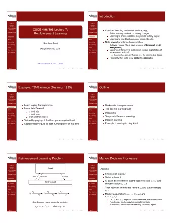
Reinforcement Learning Q-Learning Deep Q-Learning on Atari What is Reinforcement Learning? RL: general framework for online decision making given partial and delayed rewards learner is an agent that performs actions actions influence the state of the environment environment returns reward as feedback Generalization of the Multi-Armed Bandit problem

Reinforcement Learning Q-Learning Deep Q-Learning on Atari Markov Decision Processes (MDP) Models the environment that we are trying to learn Tuple ( S , A , P a , R , γ ) S the set of states (not necessarily finite) A the set of actions (not necessarily finite) P a ( s , s ′ ) the transition probability kernel R : S × A → R the reward function γ ∈ ( 0 , 1 ) the discount factor

Reinforcement Learning Q-Learning Deep Q-Learning on Atari GridWorld MDP Example States: each cell of the grid is a state Actions: move N, S, E, W, or stationary (can’t move off grid or into wall) Transitions: Deterministic, move into cell in action direction Rewards: 1 or -1 in special spots, 0 otherwise Simulation . . .

Reinforcement Learning Q-Learning Deep Q-Learning on Atari Another GridWorld Example States: each cell of the grid is a state Actions: move N, S, E, W (can’t move off grid or into wall) Transitions: Deterministic, move into cell in action direction. Any move from 10 or -100 transitions to Start. Rewards: 10 or -100 moving out of special spots, 0 otherwise

Reinforcement Learning Q-Learning Deep Q-Learning on Atari MDP Overview Example Three states S = { S 0 , S 1 , S 2 } . Two actions for each states A = { a 0 , a 1 } . Probabilistic transitions P a . Rewards defined by R : S × A → R .

Reinforcement Learning Q-Learning Deep Q-Learning on Atari Markov Property Markov Decision Processes (MDP) are very similar to Markov chains. An important property is the Markov Property . Markov Property : Set of possible actions and probability of transitions does not depend on the sequence of events that preceded it. In other words, the system is memoryless . Sometimes not completely satisfied, but approximation is good enough.

Reinforcement Learning Q-Learning Deep Q-Learning on Atari Episodic vs Continuing RL Two classes of RL problems: Episodic problems are separated by terminations and restarting, such as losing in a game and having to start over. Continuing problems are single-episode and continue forever, such as a personalized home assistance robot.

Reinforcement Learning Q-Learning Deep Q-Learning on Atari Objective Pick the actions that lead to the best future reward ”best” ← → maximize expected future discounted return: � γ t ′ − t r t ′ R t = r t + γ r t + 1 + γ 2 r t + 2 + . . . = t ′ ≥ t Discount factor γ ∈ ( 0 , 1 ) avoids infinite return encodes uncertainty about future rewards encodes bias towards immediate rewards Using a discount factor γ is only one way of capturing this.

Reinforcement Learning Q-Learning Deep Q-Learning on Atari Policy and Value Policy: π : S → P ( A ) - given a state, the probability distribution of the action the agent will choose Value: Q π ( s t , a t ) = E [ R t | s t , a t ] - given some policy π , the expected future reward under some state and action Compare to the MAB definitions: Policy: Pick an action a i . For example, UCB1 can be used to determine what action to pick. Value: The expected reward µ i associated with each action.

Reinforcement Learning Q-Learning Deep Q-Learning on Atari RL vs. Bandits Reinforcement learning is an extension of bandit problems. Standard stochastic MAB problem ← → single-state MDP . Contextual bandits can model state, but not transitions Key point: RL utilizes the entire MDP ( S , A , P a , R , γ ) . RL can account for delayed rewards and can learn to “traverse” the MDP states. No regret analysis for RL (too difficult, hard to generalize). MAB is more constrained, so it is easier to analyze and bound.

Reinforcement Learning Q-Learning Deep Q-Learning on Atari Model-based vs. Model-free RL Model-based approaches assume information about the environment Do we know the MDP (in particular its transition probabilities)? Yes: can solve MDP exactly using dynamic programming/value iteration No: try to learn the MDP (e.g. E 3 algorithm 1 ) Model-free: learn a policy in absence of a model We will focus on model-free approaches 1 Kearns and Singh (1998)

Reinforcement Learning Q-Learning Deep Q-Learning on Atari Model-free approaches Optimize either value or policy directly - or both! Value-based: Optimize value function Policy is implicit Policy-based: Optimize policy directly Value and policy based: Actor-critic 2 We will mostly consider value-based approaches. 2 Konda and Tsitsiklis 2003

Reinforcement Learning Q-Learning Deep Q-Learning on Atari Value-based RL Define optimal value function to be the best payoff among all possible policies: Q ∗ ( s , a ) = max Q π ( s , a ) π Recall π are the policies and Q π are the value functions. Value-based approaches: learn optimal value function Simple to derive a target policy from optimal value function

Reinforcement Learning Q-Learning Deep Q-Learning on Atari Exploration vs. Exploitation in RL Important concept for both RL and MAB Relevant in learning stage Fundamental tradeoff: agent should explore enough to discover a good policy, but should not sacrifice too much reward in the process ǫ -greedy strategy: Pick the ‘optimal’ strategy with probability 1 − ǫ , and select a random action with probability ǫ .

Reinforcement Learning Q-Learning Deep Q-Learning on Atari Reinforcement Learning 1 Introduction to RL. Markov Decision Processes. RL Objective and Methods. Q-Learning 2 Algorithm Example Guarantees Deep Q-Learning on Atari 3 Atari Learning Environment Deep Learning Tricks

Reinforcement Learning Q-Learning Deep Q-Learning on Atari Recall that the value function is defined as Q π ( s t , a t ) = E [ R t | s t , a t ] Recall that we can solve the RL problem by learning the optimal value function Q ∗ ( s , a ) = max Q π ( s , a ) π

Reinforcement Learning Q-Learning Deep Q-Learning on Atari Bellman equation Suppose action a leads to state s ′ . We can expand the value function recursively: Q π ( s ′ , a ′ ) | s , a ] Q π ( s , a ) = E s ′ [ r + γ max a ′ Solve using value iteration: i ( s ′ , a ′ ) | s , a ] Q π i + 1 ( s , a ) = E s ′ [ r + γ max Q π a ′

Reinforcement Learning Q-Learning Deep Q-Learning on Atari Approximating the expectation If we know the MDP’s transition probabilities, we can just write out the expectation: � Q ( s ′ , a ′ )) Q ( s , a ) = p ss ′ ( r + γ max a ′ s ′ Q-learning approximates this expectation with a single-sample iterative update (like in SGD)

Reinforcement Learning Q-Learning Deep Q-Learning on Atari Iteratively solve for optimal action-value function Q ∗ using Bellman equation updates Q ( s ′ , a ′ ) − Q ( s t , a t )] Q ( s t , a t ) = Q ( s t , a t ) + α t [ r t + γ max a ′ for learning rate α t Intuition for value iteration algorithms: a la gradient descent, iterative updates (hopefully) lead to desired convergence

Reinforcement Learning Q-Learning Deep Q-Learning on Atari Target vs. training policy We distinguish between action selection policies during training and test time. Training policy: balance exploration and exploitation such as ǫ -greedy (most commonly used) Softmax e z i σ ( z i ) = � K k = 1 e z k Target policy: pick the best possible action (highest Q-value) every time

Reinforcement Learning Q-Learning Deep Q-Learning on Atari Q-learning algorithm 1: Init Q ( s , a ) = 0 ∀ ( s , a ) inS × A 2: while not converged do t + = 1 3: pick and do action a t according to current policy (e.g. 4: ǫ -greedy) receive reward r t 5: observe new state s ′ 6: update 7: Q ( s t , a t ) = Q ( s t , a t ) + α t [ r t + γ max a ′ Q ( s ′ , a ′ ) − Q ( s t , a t )] 8: end while

Reinforcement Learning Q-Learning Deep Q-Learning on Atari On-policy vs. off-policy algorithm Q-learning is an off-policy algorithm learned Q function approximates Q ∗ independent of policy being used On-policy algorithms perform updates that depend on the policy, such as SARSA: Q ( s t , a t ) = ( 1 − α ) Q ( s t , a t ) + α t [ r t + γ Q ( s t + 1 , a t + 1 )] Convergence properties dependent on policy