Introduction CSCE CSCE 496/896 496/896 Lecture 7: Lecture 7: - PDF document

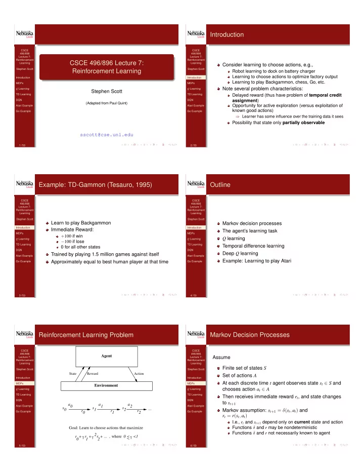
Introduction CSCE CSCE 496/896 496/896 Lecture 7: Lecture 7: Reinforcement Reinforcement CSCE 496/896 Lecture 7: Learning Learning Consider learning to choose actions, e.g., Stephen Scott Reinforcement Learning Stephen Scott Robot learning to dock on battery charger Learning to choose actions to optimize factory output Introduction Introduction Learning to play Backgammon, chess, Go, etc. MDPs MDPs Note several problem characteristics: Q Learning Q Learning Stephen Scott TD Learning TD Learning Delayed reward (thus have problem of temporal credit DQN DQN assignment ) (Adapted from Paul Quint) Opportunity for active exploration (versus exploitation of Atari Example Atari Example known good actions) Go Example Go Example ⇒ Learner has some influence over the training data it sees Possibility that state only partially observable sscott@cse.unl.edu 1 / 53 2 / 53 Example: TD-Gammon (Tesauro, 1995) Outline CSCE CSCE 496/896 496/896 Lecture 7: Lecture 7: Reinforcement Reinforcement Learning Learning Stephen Scott Stephen Scott Learn to play Backgammon Markov decision processes Introduction Introduction Immediate Reward: The agent’s learning task MDPs MDPs + 100 if win Q learning Q Learning Q Learning � 100 if lose TD Learning TD Learning Temporal difference learning 0 for all other states DQN DQN Deep Q learning Trained by playing 1.5 million games against itself Atari Example Atari Example Example: Learning to play Atari Approximately equal to best human player at that time Go Example Go Example 3 / 53 4 / 53 Reinforcement Learning Problem Markov Decision Processes CSCE CSCE 496/896 496/896 Agent Assume Lecture 7: Lecture 7: Reinforcement Reinforcement Learning Learning Finite set of states S Stephen Scott Stephen Scott State Reward Action Set of actions A Introduction Introduction At each discrete time t agent observes state s t 2 S and MDPs MDPs Environment chooses action a t 2 A Q Learning Q Learning TD Learning TD Learning Then receives immediate reward r t , and state changes DQN DQN to s t + 1 a a a 0 1 2 Atari Example Atari Example s s s ... 0 1 2 Markov assumption: s t + 1 = � ( s t , a t ) and r r r Go Example Go Example 0 1 2 r t = r ( s t , a t ) I.e., r t and s t + 1 depend only on current state and action Goal: Learn to choose actions that maximize Functions � and r may be nondeterministic Functions � and r not necessarily known to agent 2 r + γ r + r + ... , where 0 < γ <1 γ 0 1 2 5 / 53 6 / 53

Agent’s Learning Task Value Function CSCE CSCE 496/896 496/896 Lecture 7: Lecture 7: Execute actions in environment, observe results, and First consider deterministic worlds Reinforcement Reinforcement Learning Learning Learn action policy ⇡ : S ! A that maximizes For each possible policy ⇡ the agent might adopt, we Stephen Scott Stephen Scott can define discounted cumulative reward as ⇥ ⇤ r t + � r t + 1 + � 2 r t + 2 + · · · E Introduction Introduction 1 MDPs MDPs X from any starting state in S V π ( s ) ⌘ r t + � r t + 1 + � 2 r t + 2 + · · · = � i r t + i , Q Learning Q Learning Here 0  � < 1 is the discount factor for future i = 0 TD Learning TD Learning rewards DQN DQN where r t , r t + 1 , . . . are generated by following policy ⇡ , Note something new: Atari Example Atari Example starting at state s Target function is ⇡ : S ! A Go Example Go Example But we have no training examples of form h s , a i Restated, the task is to learn an optimal policy ⇡ ⇤ Training examples are of form hh s , a i , r i ⇡ ⇤ ⌘ argmax I.e., not told what best action is, instead told reward for V π ( s ) , ( 8 s ) executing action a in state s π 7 / 53 8 / 53 Value Function What to Learn CSCE CSCE We might try to have agent learn the evaluation 496/896 496/896 function V π ⇤ (which we write as V ⇤ ) Lecture 7: 0 Lecture 7: 0 100 Reinforcement Reinforcement G Learning Learning 0 It could then do a lookahead search to choose best 0 0 Stephen Scott Stephen Scott 0 0 100 action from any state s because 0 0 Introduction Introduction 0 0 ⇡ ⇤ ( s ) = argmax [ r ( s , a ) + � V ⇤ ( � ( s , a ))] , MDPs MDPs a Q Learning Q Learning r ( s , a ) values Q ( s , a ) values TD Learning TD Learning i.e., choose action that maximized immediate reward + DQN DQN G discounted reward if optimal strategy followed from G 90 100 0 Atari Example Atari Example then on Go Example Go Example E.g., V ⇤ ( bot . ctr . ) = 0 + � 100 + � 2 0 + � 3 0 + · · · = 90 81 90 100 A problem: This works well if agent knows � : S ⇥ A ! S , and V ⇤ ( s ) values One optimal policy r : S ⇥ A ! R But when it doesn’t, it can’t choose actions this way 9 / 53 10 / 53 Q Function Training Rule to Learn Q CSCE CSCE Note Q and V ⇤ closely related: 496/896 496/896 Define new function very similar to V ⇤ : Lecture 7: Lecture 7: Reinforcement Reinforcement V ⇤ ( s ) = max Q ( s , a 0 ) Learning Learning Q ( s , a ) ⌘ r ( s , a ) + � V ⇤ ( � ( s , a )) a 0 Stephen Scott Stephen Scott Which allows us to write Q recursively as Introduction Introduction i.e., Q ( s , a ) = total discounted reward if action a taken in MDPs MDPs r ( s t , a t ) + � V ⇤ ( � ( s t , a t ))) state s and optimal choices made from then on Q ( s t , a t ) = Q Learning Q Learning Q ( s t + 1 , a 0 ) If agent learns Q , it can choose optimal action even = r ( s t , a t ) + � max TD Learning TD Learning a 0 without knowing � DQN DQN Let ˆ Atari Example Atari Example Q denote learner’s current approximation to Q ; ⇡ ⇤ ( s ) [ r ( s , a ) + � V ⇤ ( � ( s , a ))] = argmax Go Example Go Example consider training rule a = Q ( s , a ) argmax ˆ ˆ Q ( s 0 , a 0 ) , Q ( s , a ) r + � max a a 0 where s 0 is the state resulting from applying action a in Q is the evaluation function the agent will learn state s 11 / 53 12 / 53

Q Learning for Deterministic Worlds Updating ˆ Q CSCE CSCE 496/896 496/896 For each s , a initialize table entry ˆ Q ( s , a ) 0 Lecture 7: Lecture 7: Reinforcement Reinforcement Learning Learning Observe current state s ˆ ˆ Q ( s 2 , a 0 ) Q ( s 1 , a right ) r + γ max 72 100 90 100 R R a 0 66 66 Stephen Scott Stephen Scott 81 81 Do forever: = 0 + 0 . 9 max { 66 , 81 , 100 } a right = 90 Select an action a (greedily or probabilistically) and Introduction Introduction Initial state: s 1 Next state: s 2 execute it MDPs MDPs Receive immediate reward r Q Learning Q Learning Can show via induction on n that if rewards non-negative Observe the new state s 0 and ˆ TD Learning TD Learning Q s initially 0, then Update the table entry for ˆ Q ( s , a ) as follows: DQN DQN ( 8 s , a , n ) ˆ Q n + 1 ( s , a ) � ˆ Atari Example Atari Example Q n ( s , a ) ˆ ˆ Q ( s , a ) r + � max Q ( s 0 , a 0 ) Go Example Go Example a 0 and s s 0 ( 8 s , a , n ) 0  ˆ Q n ( s , a )  Q ( s , a ) Note that actions not taken and states not seen don’t get explicit updates (might need to generalize) 13 / 53 14 / 53 Updating ˆ Updating ˆ Q Q Convergence Convergence CSCE CSCE 496/896 496/896 For any table entry ˆ Q n ( s , a ) updated on iteration n + 1 , Lecture 7: Lecture 7: ˆ Q converges to Q : Consider case of deterministic Reinforcement Reinforcement error in the revised estimate ˆ Q n + 1 ( s , a ) is Learning Learning world where each h s , a i is visited infinitely often Stephen Scott Stephen Scott | ˆ ˆ Q n + 1 ( s , a ) � Q ( s , a ) | = | ( r + � max Q n ( s 0 , a 0 )) Proof : Define a full interval to be an interval during a 0 Introduction Introduction which each h s , a i is visited. Will show that during each � ( r + � max Q ( s 0 , a 0 )) | MDPs MDPs full interval the largest error in ˆ Q table is reduced by a 0 Q Learning Q Learning ˆ Q n ( s 0 , a 0 ) � max Q ( s 0 , a 0 ) | = � | max factor of � TD Learning TD Learning a 0 a 0 Let ˆ Q n be table after n updates, and ∆ n be the | ˆ DQN DQN ( ⇤ )  � max Q n ( s 0 , a 0 ) � Q ( s 0 , a 0 ) | maximum error in ˆ a 0 Q n ; i.e., Atari Example Atari Example s 00 , a 0 | ˆ ( ⇤⇤ )  � max Q n ( s 00 , a 0 ) � Q ( s 00 , a 0 ) | Go Example Go Example s , a | ˆ ∆ n = max Q n ( s , a ) � Q ( s , a ) | = � ∆ n Let s 0 = � ( s , a ) ( ⇤ ) works since | max a f 1 ( a ) � max a f 2 ( a ) |  max a | f 1 ( a ) � f 2 ( a ) | ( ⇤⇤ ) works since max will not decrease 15 / 53 16 / 53 Updating ˆ Q Nondeterministic Case Convergence CSCE CSCE What if reward and next state are non-deterministic? 496/896 496/896 Lecture 7: Lecture 7: Reinforcement Reinforcement We redefine V , Q by taking expected values: Learning Learning Stephen Scott Stephen Scott ⇥ ⇤ r t + � r t + 1 + � 2 r t + 2 + · · · V π ( s ) ⌘ E Also, ˆ Q 0 ( s , a ) and Q ( s , a ) are both bounded 8 s , a " 1 # Introduction Introduction X ) ∆ 0 bounded � i r t + i MDPs MDPs = E Q Learning Thus after k full intervals, error  � k ∆ 0 Q Learning i = 0 TD Learning TD Learning Finally, each h s , a i visited infinitely often ) number of DQN DQN intervals infinite, so ∆ n ! 0 as n ! 1 E [ r ( s , a ) + � V ⇤ ( � ( s , a ))] Q ( s , a ) ⌘ Atari Example Atari Example Go Example Go Example E [ r ( s , a )] + � E [ V ⇤ ( � ( s , a ))] = X P ( s 0 | s , a ) V ⇤ ( s 0 ) = E [ r ( s , a )] + � s 0 X P ( s 0 | s , a ) max Q ( s 0 , a 0 ) = E [ r ( s , a )] + � a 0 s 0 17 / 53 18 / 53