Linear Programming Instructor: Haifeng Xu Slides of this lecture is - PowerPoint PPT Presentation
CS6501: T opics in Learning and Game Theory (Fall 2019) Linear Programming Instructor: Haifeng Xu Slides of this lecture is adapted from Shaddin Dughmi at https://www-bcf.usc.edu/~shaddin/cs675sp18/index.html Outline Linear Programing
CS6501: T opics in Learning and Game Theory (Fall 2019) Linear Programming Instructor: Haifeng Xu Slides of this lecture is adapted from Shaddin Dughmi at https://www-bcf.usc.edu/~shaddin/cs675sp18/index.html
Outline Ø Linear Programing Basics Ø Dual Program of LP and Its Properties 2
Mathematical Optimization Ø The task of selecting the best configuration from a “feasible” set to optimize some objective minimize (or maximize) 𝑔(𝑦) 𝑦 ∈ 𝑌 subject to 𝑦 : decision variable • 𝑔(𝑦) : objective function • 𝑌 : feasible set/region • • Optimal solution, optimal value Ø Example 1: minimize 𝑦 ' , s.t. 𝑦 ∈ [−1,1] Ø Example 2: pick a road to school 3
Polynomial-Time Solvability Ø A problem can be solved in polynomial time if there exists an algorithm that solves the problem in time polynomial in its input size Ø Why care about polynomial time? Why not quadratic or linear? • There are studies on fined-grained complexity • But poly-time vs exponential time seems a fundamental separation between easy and difficult problems • In many cases, after a poly-time algorithm is developed, researchers can quickly reduce the polynomial degree to be small (e.g., solving LPs) Ø In algorithm analysis, a significant chunk of research is devoted to studying the complexity of a problem by proving it is poly- time solvable or not (e.g., NP-hard problems) 4
minimize (or maximize) 𝑔(𝑦) 𝑦 ∈ 𝑌 subject to Ø Difficult to solve without any assumptions on 𝑔(𝑦) and 𝑌 Ø A ubiquitous and well-understood case is linear program 5
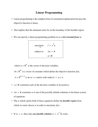
Linear Program (LP) – General Form minimize (or maximize) 𝑑 . ⋅ 𝑦 subject to 𝑏 1 ⋅ 𝑦 ≤ 𝑐 1 ∀𝑗 ∈ 𝐷 7 𝑏 1 ⋅ 𝑦 ≥ 𝑐 1 ∀𝑗 ∈ 𝐷 ' 𝑏 1 ⋅ 𝑦 = 𝑐 1 ∀𝑗 ∈ 𝐷 : Ø Decision variable: 𝑦 ∈ ℝ < Ø Parameters: • 𝑑 ∈ ℝ < define the linear objective • 𝑏 1 ∈ ℝ < and 𝑐 1 ∈ ℝ defines the 𝑗 ’th linear constraint 6
Linear Program (LP) – Standard Form maximize 𝑑 . ⋅ 𝑦 subject to 𝑏 1 ⋅ 𝑦 ≤ 𝑐 1 ∀𝑗 = 1, ⋯ , 𝑛 𝑦 ? ≥ 0 ∀𝑘 = 1, ⋯ , 𝑜 Claim. Every LP can be transformed to an equivalent standard form Ø minimize 𝑑 . ⋅ 𝑦 maximize −𝑑 . ⋅ 𝑦 ⇔ Ø 𝑏 1 ⋅ 𝑦 ≥ 𝑐 1 ⇔ −𝑏 1 ⋅ 𝑦 ≤ −𝑐 1 Ø 𝑏 1 ⋅ 𝑦 = 𝑐 1 ⇔ 𝑏 1 ⋅ 𝑦 ≤ 𝑐 1 and −𝑏 1 ⋅ 𝑦 ≤ −𝑐 1 D − 𝑦 ? E ≥ 0 E with 𝑦 ? D , 𝑦 ? Ø Any unconstrained 𝑦 ? can be replaced by 𝑦 ? 7
Geometric Interpretation 𝑑 𝑑 ⋅ 𝑦 = 𝑤 𝑏 1 ⋅ 𝑦 = 𝑐 1 8
Geometric Interpretation 𝑑 𝑑 ⋅ 𝑦 = 𝑤 𝑏 1 ⋅ 𝑦 = 𝑐 1 9
A 2-D Example 10
Application: Optimal Production Ø 𝑜 products, 𝑛 raw materials Ø Every unit of product 𝑘 uses 𝑏 1? units of raw material 𝑗 Ø There are 𝑐 1 units of material 𝑗 available Ø Product 𝑘 yields profit 𝑑 ? per unit Ø Factory wants to maximize profit subject to available raw materials 𝑘 : product index 𝑗 : material index maximize 𝑑 . ⋅ 𝑦 subject to 𝑏 1 ⋅ 𝑦 ≤ 𝑐 1 ∀𝑗 = 1, ⋯ , 𝑛 𝑦 ? ≥ 0 ∀𝑘 = 1, ⋯ , 𝑜 where variable 𝑦 ? = # units of product 𝑘 11
Terminology Ø Hyperplane: The region defined by a linear equality 𝑏 1 ⋅ 𝑦 = 𝑐 1 Ø Halfspace: The region defined by a linear inequality 𝑏 1 ⋅ 𝑦 ≤ 𝑐 1 Ø Polyhedron: The intersection of a set of linear inequalities • Feasible region of an LP is a polyhedron Ø Polytope: Bounded polyhedron Ø Vertex: A point 𝑦 is a vertex of polyhedron 𝑄 if ∄ 𝑧 ≠ 0 with 𝑦 + 𝑧 ∈ 𝑄 and 𝑦 − 𝑧 ∈ 𝑄 Red point: vertex Blue point: not a vertex 12
Terminology Convex set: A set 𝑇 is convex if ∀𝑦, 𝑧 ∈ 𝑇 and ∀𝑞 ∈ [0,1] , we have 𝑞 ⋅ 𝑦 + 1 − 𝑞 ⋅ 𝑧 ∈ 𝑇 Ø Inherently related to convex functions convex Non-convex 13
Terminology Convex set: A set 𝑇 is convex if ∀𝑦, 𝑧 ∈ 𝑇 and ∀𝑞 ∈ [0,1] , we have 𝑞 ⋅ 𝑦 + 1 − 𝑞 ⋅ 𝑧 ∈ 𝑇 Convex hull: the convex hull of points x 7 , ⋯ , 𝑦 O ∈ ℝ is < < 𝑡. 𝑢. ∑𝑞 1 = 1 convhull 𝑦 7 , ⋯ , 𝑦 < = x = W 𝑞 1 𝑦 1 : ∀𝑞 ∈ ℝ D 1X7 That is, convhull 𝑦 7 , ⋯ , 𝑦 < includes all points that can be written as expectation of 𝑦 7 , ⋯ , 𝑦 < under some distribution 𝑞 . Ø Any polytope (i.e., a bounded polyhedron) is the convex hull of a finite set of points Geometric visualization of convex hull 14
Basic Facts about LPs and Polyhedrons Fact : The feasible region of any LP (a polyhedron) is a convex set. All possible objective values form an interval (possibly unbounded). Note: intervals are the only convex sets in ℝ Any 𝑤 ∈ [𝑤 7 , 𝑤 ' ] must also be a possible objective value 𝑑 ⋅ 𝑑 𝑦 ⋅ = 𝑦 = 𝑤 𝑤 7 ' 15
Basic Facts about LPs and Polyhedrons Fact : The feasible region of any LP (a polyhedron) is a convex set. All possible objective values form an interval (possibly unbounded). Note: intervals are the only convex sets in ℝ Fact : The set of optimal solutions of any LP is a convex set. Ø It is the intersection of feasible region and hyperplane 𝑑 . ⋅ 𝑦 = 𝑃𝑄𝑈 Fact : At a vertex, 𝑜 linearly independent constraints are satisfied with equality (a.k.a., tight). Formal proofs: homework exercise 16
Basic Facts about LPs and Polyhedrons Fact : An LP either has an optimal solution, or is unbounded or infeasible 𝑑 17
Basic Facts about LPs and Polyhedrons Fact : An LP either has an optimal solution, or is unbounded or infeasible 𝑑 18
Basic Facts about LPs and Polyhedrons Fact : An LP either has an optimal solution, or is unbounded or infeasible 𝑑 19
̅ ̅ ̅ ̅ Fundamental Theorem of LP Theorem : if an LP in standard form has an optimal solution, then it has a vertex optimal solution. Proof 𝑦 with the Ø Assume not, and take a non-vertex optimal solution ̅ maximum number of tight constraints Ø There is 𝑧 ≠ 0 s.t. ̅ 𝑦 ± 𝑧 are feasible Ø 𝑧 is orthogonal to objective function and all tight constraints at ̅ 𝑦 . ⋅ 𝑧 = 0 whenever the 𝑗 ’th constraint is tight for ̅ i.e. 𝑑 . ⋅ 𝑧 = 0 , and 𝑏 1 𝑦 • . ⋅ 𝑧 = 0 Arguments for 𝑏 1 a) . ⋅ 𝑦 ± 𝑧 feasible ⇒ 𝑏 1 𝑦 ± 𝑧 ≤ 𝑐 1 • . ⋅ ̅ 𝑦 is tight at constraint 𝑗 ⇒ 𝑏 1 𝑦 = 𝑐 1 • . ⋅ ± 𝑧 ≤ 0 ⇒ 𝑏 1 . ⋅ 𝑧 = 0 These together yield 𝑏 1 • 𝑦 ± 𝑧 ≤ 𝑑 . ̅ 𝑦 optimal implies 𝑑 . 𝑦 ⇒ 𝑑 c 𝑧 = 0 b) Similarly, ̅ 20
Fundamental Theorem of LP Theorem : if an LP in standard form has an optimal solution, then it has a vertex optimal solution. Proof Ø Assume not, and take a non-vertex optimal solution 𝑦 with the maximum number of tight constraints Ø There is 𝑧 ≠ 0 s.t. 𝑦 ± 𝑧 are feasible Ø 𝑧 is orthogonal to objective function and all tight constraints at 𝑦 . ⋅ 𝑧 = 0 whenever the 𝑗 ’th constraint is tight for 𝑦 i.e. 𝑑 . ⋅ 𝑧 = 0 , and 𝑏 1 • Ø Can choose 𝑧 s.t. 𝑧 ? < 0 for some 𝑘 Ø Let 𝛽 be the largest constant such that 𝑦 + 𝛽𝑧 is feasible Such an 𝛽 exists (since 𝑦 ? + 𝛽𝑧 ? < 0 if 𝛽 very large) • Ø An additional constraint becomes tight at 𝑦 + 𝛽𝑧 , contradiction 21
Fundamental Theorem of LP Theorem : if an LP in standard form has an optimal solution, then it has a vertex optimal solution. Corollary [counting non-zero variables]: If an LP in standard form has an optimal solution, then there is an optimal solution with at most 𝑛 non-zero variables. maximize 𝑑 . ⋅ 𝑦 subject to 𝑏 1 ⋅ 𝑦 ≤ 𝑐 1 ∀𝑗 = 1, ⋯ , 𝑛 𝑦 ? ≥ 0 ∀𝑘 = 1, ⋯ , 𝑜 Ø Meaningful when 𝑛 < 𝑜 Ø E.g. for optimal production with 𝑜 = 10 products and 𝑛 = 3 raw materials, there is an optimal plan using at most 3 products . 22
Poly-Time Solvability of LP Theorem : any linear program with 𝑜 variables and 𝑛 constraints can be solved in poly(𝑛, 𝑜) time. Ø Original proof gives an algorithm with very high polynomial degree Ø Now, the fastest algorithm with guarantee takes min(𝑜, 𝑛) ⋅ 𝑈 where 𝑈 = time of solving linear equation systems of the same size Ø In practice, Simplex Algorithm runs extremely fast though in (extremely rare) worst case it still takes exponential time Ø We will not cover these algorithms; Instead, we use them as building blocks to solve other problems 23
Brief History of Linear Optimization Ø The forefather of convex optimization problems, and the most ubiquitous. Ø Developed by Kantorovich during World War II (1939) for planning the Soviet army’s expenditures and returns. Kept secret. Ø Discovered a few years later by George Dantzig, who in 1947 developed the simplex method for solving linear programs Ø John von Neumann developed LP duality in 1947, and applied it to game theory Ø Polynomial-time algorithms: Ellipsoid method (Khachiyan 1979), interior point methods (Karmarkar 1984). 24
Outline Ø Linear Programing Basics Ø Dual Program of LP and Its Properties 25
Recommend
More recommend
Explore More Topics
Stay informed with curated content and fresh updates.
