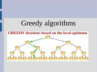
Greedy Algorithms Algorithm Theory WS 2013/14 Fabian Kuhn Greedy - - PowerPoint PPT Presentation

Chapter 2

Greedy Algorithms

Algorithm Theory WS 2013/14 Fabian Kuhn

Algorithm Theory, WS 2013/14 Fabian Kuhn 2

Greedy Algorithms

• No clear definition, but essentially:
• Depending on problem, greedy algorithms can give

– Optimal solutions – Close to optimal solutions – No (reasonable) solutions at all

• If it works, very interesting approach!

– And we might even learn something about the structure of the problem

Goal: Improve understanding where it works (mostly by examples) In each step make the choice that looks best at the moment!

Algorithm Theory, WS 2013/14 Fabian Kuhn 3

Interval Scheduling

• Given: Set of intervals, e.g.

[0,10],[1,3],[1,4],[3,5],[4,7],[5,8],[5,12],[7,9],[9,12],[8,10],[11,14],[12,14]

• Goal: Select largest possible non‐overlapping set of intervals

– Overlap at boundary ok, i.e., [4,7] and [7,9] are non‐overlapping

• Example: Intervals are room requests; satisfy as many as possible

1 2 3 4 5 7 6 8 9 10 11 12 13 14 [0,10] [0,10] [1,3] [1,3] [1,4] [1,4] [3,5] [3,5] [4,7] [4,7] [5,8] [5,8] [11,14] [11,14] [5,12] [5,12] [8,10] [8,10] [12,14] [12,14] [7,9] [7,9] [9,12] [9,12]

Algorithm Theory, WS 2013/14 Fabian Kuhn 4

Greedy Algorithms

• Several possibilities…

Choose first available interval: Choose shortest available interval:

1 2 3 4 5 7 6 8 9 10 11 12 13 14 [0,10] [0,10] [1,3] [1,3] [1,4] [1,4] [3,5] [3,5] [4,7] [4,7] [5,8] [5,8] [11,14] [11,14] [5,12] [5,12] [8,10] [8,10] [12,14] [12,14] 1 2 3 4 5 7 6 8 9 10 11 12 13 14 [6,9] [1,7] [1,7] [8,14] [8,14] [7,9] [7,9] [9,12] [9,12]

Algorithm Theory, WS 2013/14 Fabian Kuhn 5

Greedy Algorithms

Choose available request with earliest finishing time: ≔ set of all requests; ≔ empty set; while is not empty do choose ∈ with smallest finishing time add to delete all requests from that are not compatible with end // is the solution

1 2 3 4 5 7 6 8 9 10 11 12 13 14 [0,10] [0,10] [1,3] [1,3] [1,4] [1,4] [3,5] [3,5] [4,7] [4,7] [5,8] [5,8] [11,14] [11,14] [5,12] [5,12] [7,9] [7,9] [8,10] [8,10] [12,14] [12,14] [1,3] [1,3] [3,5] [3,5] [5,8] [5,8] [11,14] [11,14] [8,10] [8,10] [9,12] [9,12]

Algorithm Theory, WS 2013/14 Fabian Kuhn 6

Earliest Finishing Time is Optimal

• Let be the set of intervals of an optimal solution
• Can we show that ?

– No…

• Show that .

1 2 3 4 5 7 6 8 9 10 11 12 13 14 [0,10] [0,10] [1,3] [1,3] [1,4] [1,4] [3,5] [3,5] [4,7] [4,7] [5,8] [5,8] [11,14] [11,14] [5,12] [5,12] [8,10] [8,10] [12,14] [12,14] [7,9] [7,9] [9,12] [9,12] Greey Solution Greey Solution Alternative Optimal Sol. Alternative Optimal Sol.

Algorithm Theory, WS 2013/14 Fabian Kuhn 7

Greedy Stays Ahead

• Greedy Solution:

, , , , … , , , where

• Optimal Solution:
• ∗,

∗ , ∗, ∗ , … , ∗ , ∗

, where

∗ ∗

• Assume that ∞ for || and

∗ ∞ for ||

Claim: For all 1,

∗

1 2 3 4 5 7 6 8 9 10 11 12 13 14 [0,10] [0,10] [1,3] [1,3] [1,4] [1,4] [3,5] [3,5] [4,7] [4,7] [5,8] [5,8] [11,14] [11,14] [5,12] [5,12] [8,10] [8,10] [12,14] [12,14] [7,9] [7,9] [9,12] [9,12]

Algorithm Theory, WS 2013/14 Fabian Kuhn 8

Greedy Stays Ahead

Claim: For all 1,

∗

Proof (by induction on ): Corollary: Earliest finishing time algorithm is optimal.

Algorithm Theory, WS 2013/14 Fabian Kuhn 9

Weighted Interval Scheduling

Weighted version of the problem:

• Each interval has a weight
• Goal: Non‐overlapping set with maximum total weight

Earliest finishing time greedy algorithm fails:

• Algorithm needs to look at weights
• Else, the selected sets could be the ones with smallest weight…

No simple greedy algorithm:

• We will see an algorithm using another design technique later.

Algorithm Theory, WS 2013/14 Fabian Kuhn 10

Interval Partitioning

• Schedule all intervals: Partition intervals into as few as

possible non‐overlapping sets of intervals

– Assign intervals to different resources, where each resource needs to get a non‐overlapping set

• Example:

– Intervals are requests to use some room during this time – Assign all requests to some room such that there are no conflicts – Use as few rooms as possible

• Assignment to 3 resources:

[1,3] [1,3] [1,4] [1,4] [2,4] [2,4] [4,7] [4,7] [5,8] [5,8] [5,12] [5,12] [9,11] [9,11] [12,14] [12,14] [9,12] [9,12]

Algorithm Theory, WS 2013/14 Fabian Kuhn 11

Depth

Depth of a set of intervals:

• Maximum number passing over a single point in time
• Depth of initial example is 4 (e.g., [0,10],[4,7],[5,8],[5,12]):

Lemma: Number of resources needed depth

1 2 3 4 5 7 6 8 9 10 11 12 13 14 [0,10] [0,10] [1,3] [1,3] [1,4] [1,4] [3,5] [3,5] [4,7] [4,7] [5,8] [5,8] [11,14] [11,14] [5,12] [5,12] [8,10] [8,10] [12,14] [12,14] [7,9] [7,9] [9,12] [9,12]

Algorithm Theory, WS 2013/14 Fabian Kuhn 12

Greedy Algorithm

Can we achieve a partition into “depth” non‐overlapping sets?

• Would mean that the only obstacles to partitioning are local…

Algorithm:

• Assigns labels 1, … to the sets; same label  non‐overlapping

1. sort intervals by starting time: , , … , 2. for 1 to do 3. assign smallest possible label to (possible label: different from conflicting intervals

, )

4. end

Algorithm Theory, WS 2013/14 Fabian Kuhn 13

Interval Partitioning Algorithm

Example:

• Labels:
• Number of labels = depth = 4

1 2 3 4 5 7 6 8 9 10 11 12 13 14 [0,10] [0,10] [1,3] [1,3] [1,4] [1,4] [3,5] [3,5] [4,7] [4,7] [5,8] [5,8] [11,14] [11,14] [5,12] [5,12] [8,10] [8,10] [12,14] [12,14] [7,9] [7,9] [9,12] [9,12] [0,10] [0,10] [0,10] [0,10] [1,3] [1,3] [1,4] [1,4] [3,5] [3,5] [4,7] [4,7] [5,8] [5,8] [5,12] [5,12] [7,9] [7,9] [8,10] [8,10] [9,12] [9,12] [11,14] [11,14] [12,14] [12,14]

Algorithm Theory, WS 2013/14 Fabian Kuhn 14

Interval Partitioning: Analysis

Theorem: a) Let be the depth of the given set of intervals. The algorithm assigns a label from 1, … , to each interval. b) Sets with the same label are non‐overlapping Proof:

• b) holds by construction
• For a):

– All intervals

, overlapping with , overlap at the beginning of

– At most 1 such intervals  some label in 1, … , is available.

Algorithm Theory, WS 2013/14 Fabian Kuhn 15

Traveling Salesperson Problem (TSP)

Input:

• Set of nodes (points, cities, locations, sites)
• Distance function : → , i.e., , : dist. from to
• Distances usually symmetric, asymm. distances  asymm. TSP

Solution:

• Ordering/permutation , , … , of nodes
• Length of TSP path: ∑

,

• Length of TSP tour: , ∑

,

• Goal:
• Minimize length of TSP path or TSP tour

Algorithm Theory, WS 2013/14 Fabian Kuhn 16

Example

3 13 4 9 1 10 32 33 3 3 8 2 20 21 18 17 1 19 9 1 6 2 2

Optimal Tour: Length: 86 Greedy Algorithm? Length: 121

Algorithm Theory, WS 2013/14 Fabian Kuhn 17

Nearest Neighbor (Greedy)

• Nearest neighbor can be arbitrarily bad, even for TSP paths

1 1000 2 1 2 2

Algorithm Theory, WS 2013/14 Fabian Kuhn 18

TSP Variants

• Asymmetric TSP

– arbitrary non‐negative distance/cost function – most general, nearest neighbor arbitrarily bad – NP‐hard to get within any bound of optimum

• Symmetric TSP

– arbitrary non‐negative distance/cost function – nearest neighbor arbitrarily bad – NP‐hard to get within any bound of optimum

• Metric TSP

– distance function defines metric space: symmetric, non‐negative, triangle inequality: , , , – possible to get close to optimum (we will later see factor ⁄ ) – what about the nearest neighbor algorithm?

Algorithm Theory, WS 2013/14 Fabian Kuhn 19

Metric TSP, Nearest Neighbor

Optimal TSP tour: Nearest‐Neighbor TSP tour: 1 2 3 4 5 6 7 9 8 10 11 12

1.3 1.1 2.1 0.8 1.9 4.0 2.1 1.3 1.2 3.4 3.1 1.7

Algorithm Theory, WS 2013/14 Fabian Kuhn 20

Metric TSP, Nearest Neighbor

Optimal TSP tour: Nearest‐Neighbor TSP tour: cost = 24 1 2 3 4 5 6 7 9 8 10 11 12

1.3 1.1 2.1 0.8 1.9 4.0 2.1 1.3 1.2 3.4 3.1 1.7

Algorithm Theory, WS 2013/14 Fabian Kuhn 21

Metric TSP, Nearest Neighbor

Triangle Inequality:

• ptimal tour on remaining nodes
• verall optimal tour

7 9 10 11 12

2.1 1.3 3.4 3.1 1.7

Algorithm Theory, WS 2013/14 Fabian Kuhn 22

Metric TSP, Nearest Neighbor

Analysis works in phases:

• In each phase, assign each optimal edge to some greedy edge

– Cost of greedy edge cost of optimal edge

• Each greedy edge gets assigned 2 optimal edges

– At least half of the greedy edges get assigned

• At end of phase:

Remove points for which greedy edge is assigned Consider optimal solution for remaining points

• Triangle inequality: remaining opt. solution overall opt. sol.
• Cost of greedy edges assigned in each phase opt. cost
• Number of phases

– +1 for last greedy edge in tour

Algorithm Theory, WS 2013/14 Fabian Kuhn 23

Metric TSP, Nearest Neighbor

• Assume:

NN: cost of greedy tour, OPT: cost of optimal tour

• We have shown:

NN OPT 1 log

• Example of an approximation algorithm
• We will later see a

⁄ ‐approximation algorithm for metric TSP

Algorithm Theory, WS 2013/14 Fabian Kuhn 24

Back to Scheduling

• Given: requests / jobs with deadlines:
• Goal: schedule all jobs with minimum lateness

– Schedule: , : start and finishing times of request Note:

• Lateness ≔ max 0, max
• – largest amount of time by which some job finishes late
• Many other natural objective functions possible…

1 2 3 4 5 7 6 8 9 10 11 12 13 14 length 10 length 10 3 3 5 5 7 7 deadline 11 10 13 7

Algorithm Theory, WS 2013/14 Fabian Kuhn 25

Greedy Algorithm?

Schedule jobs in order of increasing length?

• Ignores deadlines: seems too simplistic…
• E.g.:

Schedule by increasing slack time?

• Should be concerned about slack time:

10 10 deadline 10 ⋯ 100 2 2 2 2 10 10 Schedule: 10 10 deadline 10 3 2 2 2 2 10 10 Schedule:

Algorithm Theory, WS 2013/14 Fabian Kuhn 26

Greedy Algorithm

Schedule by earliest deadline?

• Schedule in increasing order of
• Ignores lengths of jobs: too simplistic?
• Earliest deadline is optimal!

Algorithm:

• Assume jobs are reordered such that ⋯
• Start/finishing times:

– First job starts at time 1 0 – Duration of job is : – No gaps between jobs: 1

(idle time: gaps in a schedule  alg. gives schedule with no idle time)

Algorithm Theory, WS 2013/14 Fabian Kuhn 27

Example

Jobs ordered by deadline: Schedule: Lateness: job 1: 0, job 2: 0, job 3: 4, job 4: 5

1 2 3 4 5 7 6 8 9 10 11 12 13 14 7 7 3 3 5 5 3 3 11 10 13 7 1 2 3 4 5 7 6 8 9 10 11 12 13 14 5 5 3 3 7 7 3 3

Algorithm Theory, WS 2013/14 Fabian Kuhn 28

Basic Facts

• 1. There is an optimal schedule with no idle time

– Can just schedule jobs earlier…

• 2. Inversion: Job scheduled before job if

Schedules with no inversions have the same maximum lateness

Algorithm Theory, WS 2013/14 Fabian Kuhn 29

Earliest Deadline is Optimal

Theorem: There is an optimal schedule with no inversions and no idle time. Proof:

• Consider optimal schedule ′ with no idle time
• If ′ has inversions, ∃ pair , , s.t. is scheduled immediately

before and

• Claim: Swapping and gives schedule with

1. Less inversions 2. Maximum lateness no larger than in ′

Algorithm Theory, WS 2013/14 Fabian Kuhn 30

Earliest Deadline is Optimal

Claim: Swapping and : maximum lateness no larger than in ′

Algorithm Theory, WS 2013/14 Fabian Kuhn 31

Exchange Argument

• General approach that often works to analyze greedy algorithms
• Start with any solution
• Define basic exchange step that allows to transform solution into

a new solution that is not worse

• Show that exchange step move solution closer to the solution

produced by the greedy algorithm

• Number of exchange steps to reach greedy solution should be

finite…

Algorithm Theory, WS 2013/14 Fabian Kuhn 32

Another Exchange Argument Example

• Minimum spanning tree (MST) problem

– Classic graph‐theoretic optimization problem

• Given: weighted graph
• Goal: spanning tree with min. total weight
• Several greedy algorithms work
• Kruskal’s algorithm:

– Start with empty edge set – As long as we do not have a spanning tree: add minimum weight edge that doesn’t close a cycle

Algorithm Theory, WS 2013/14 Fabian Kuhn 33

Kruskal Algorithm: Example

3 14 4 6 1 10 13 23 21 31 8 25 20 11 18 17 16 19 9 12 7 2 28

Algorithm Theory, WS 2013/14 Fabian Kuhn 34

Kruskal is Optimal

• Basic exchange step: swap to edges to get from tree to tree ′

– Swap out edge not in Kruskal tree, swap in edge in Kruskal tree – Swapping does not increase total weight

• For simplicity, assume, weights are unique:

Algorithm Theory, WS 2013/14 Fabian Kuhn 35

Matroids

• Same, but more abstract…

Matroid: pair ,

• : set, called the ground set
• : finite family of finite subsets of (i.e., ⊆ 2),

called independent sets , needs to satisfy 3 properties:

• 1. Empty set is independent, i.e., ∅ ∈ (implies that ∅)
• 2. Hereditary property: For all ⊆ and all ⊆ ,

if ∈ , then also ∈

• 3. Augmentation / Independent set exchange property:

If , ∈ and ||, there exists ∈ ∖ such that ≔ ∪ ∈

Algorithm Theory, WS 2013/14 Fabian Kuhn 36

Example

• Fano matroid:

– Smallest finite projective plane of order 2…

Algorithm Theory, WS 2013/14 Fabian Kuhn 37

Matroids and Greedy Algorithms

Weighted matroid: each ∈ has a weight 0 Goal: find maximum weight independent set Greedy algorithm:

• 1. Start with ∅
• 2. Add max. weight ∈ ∖ to such that ∪ ∈

Claim: greedy algorithm computes optimal solution

Algorithm Theory, WS 2013/14 Fabian Kuhn 38

Greedy is Optimal

• : greedy solution : any other solution

Algorithm Theory, WS 2013/14 Fabian Kuhn 39

Matroids: Examples

Forests of a graph , :

• forest : subgraph with no cycles (i.e., ⊆ )
• : set of all forests  , is a matroid
• Greedy algorithm gives maximum weight forest

(equivalent to MST problem) Bicircular matroid of a graph , :

• : set of edges such that every connected subset has 1 cycle
• , is a matroid  greedy gives max. weight such subgraph

Linearly independent vectors:

• Vector space , : finite set of vectors, : sets of lin. indep. vect.
• Fano matroid can be defined like that

Algorithm Theory, WS 2013/14 Fabian Kuhn 40

Greedoid

• Matroids can be generalized even more
• Relax hereditary property:

Replace ⊆ ⊆ ⟹ ∈ by ∅ ⊆ ⟹ ∃ ∈ , s. t. ∖ ∈

• Exchange property holds as before
• Under certain conditions on the weights, greedy is optimal for

computing the max. weight ∈ of a greedoid.

– Additional conditions automatically satisfied by hereditary property

• More general than matroids